Paper

Size-based scheduling for message queues, from per-key duration statistics.

Divyanshu Singh. The full write-up, with the design, the pre-registered evaluation and the limits.

Abstract

In most message queues one slow job delays every cheap job behind it. Priorities fix this only if someone knows each job’s cost and keeps the map current. Harbinger is a gRPC broker that removes that step: it learns how long each kind of message takes from the acknowledgements it already receives, and serves short expected work first. On a production-style job queue it cut mean latency by 30.8% against FIFO on AWS and beat a hand-tuned priority map, and as a sidecar the same predictor cut RabbitMQ’s mean latency by 57.6%. Much of this came from plain per-key duration statistics, with no model to train. Under long backlogs, though, the broker’s own default aging gave most of the gain back wherever we tested it, and only a design with worker-time weights and pausing aging passed on replayed Azure and Huawei traces, at high load (Azure is in-sample for that design). Other ideas did not pay off: size-binned keys and learned models added nothing reliable, a queue per job type beat prediction on mean latency, tail latency never improved, and on two HPC logs prediction gave no gain on one and made the other worse. All pass criteria were frozen before the runs, but the evidence is synthetic or trace-driven: in the trace replays each job simply waits out its recorded duration instead of doing real work, so they test the scheduling but not the contention real handlers would cause. We claim no production readiness.

1 Introduction

Almost every large service is built around queues. A web request that would take too long to finish synchronously becomes a message, and a pool of workers picks it up later. Cloud vendors document the pattern as a design pattern, because a queue between a task and the service it calls smooths bursts of demand that would otherwise overload the service (Microsoft 2026b), and serverless platforms use it to connect functions to the rest of the cloud, with a managed fleet of pollers that read from a queue and invoke a function for each batch of messages (Amazon Web Services 2026b). Inside large companies it runs at a scale that is hard to picture: Meta describes an internal queueing service that processes close to a trillion items a day, on behalf of notifications, integrity checks, video encoding and the many other tasks that microservices hand to one another asynchronously (Nanavati and Joshi 2021). Queues also carry the machinery of reliability, namely retries, separate retry queues so that one bad message does not block a batch, and dead-letter queues for the messages that never succeed (Uber Engineering 2018). When the work behind a service is not what a user is waiting on, it is in a queue.

The trouble is that one queue usually carries very different kinds of work. A notification that takes a few milliseconds shares a queue, and often a pool of workers, with a report export that takes tens of seconds, and when load rises the cheap job waits behind the expensive one. This is head-of-line blocking, the same mechanism that makes tail latency so hard to control in interactive services (Dean and Barroso 2013), and a known concern for microservice applications in which many such calls compose (Gan et al. 2019). It hurts the mean and the median as well as the tail, because most jobs are the cheap ones.

Practitioners have a standard answer, which is to prioritise. The Azure Architecture Center describes a pattern in which the producer assigns each message a priority and consumers handle higher priorities first, or in which separate queues are kept per priority (Microsoft 2026a); Meta’s queue and RabbitMQ also let producers set a priority on every item (Nanavati and Joshi 2021; RabbitMQ 2026), whereas SQS offers standard and FIFO queues but no priority (Amazon Web Services 2026a) and a Kafka partition is consumed in offset order (Kreps et al. 2011). Even where priorities exist, they put the burden on a person. Someone has to know what each endpoint costs, decide where it belongs, and revisit that decision when code or traffic changes, and getting it wrong is not harmless: in our benchmark a plausible but misconfigured map was slower than doing nothing at all, by 6.6% locally and 9.4% on AWS.

Scheduling theory suggests a route that needs no such person. If a job’s processing time is known, serving the shortest first minimises mean response time (Schrage 1968), and that idea has been put to work in web servers (Harchol-Balter et al. 2003), data-processing clusters (Pastorelli et al. 2013) and GPU cluster managers (Gu et al. 2019). All of these assume that the scheduler knows a job’s size or can watch the job run. A message broker can do neither. The handler is arbitrary code behind a network call, it cannot be preempted, and nobody declared its cost. This gap is what the paper addresses.

What a broker can do is remember. It delivers every message and receives the acknowledgement, so it can measure how long each kind of message actually took and use that history to predict the next one. We build this into Harbinger. For each message key, the producer optionally joined to a job-type header, the broker keeps a decaying histogram of handler durations reported on acknowledgement, looks up the key’s expected duration when a message arrives, and places the message in one of a few priority levels. A key with too little, too old or too variable a history goes to a default level instead. Nothing is trained and the operator configures no per-endpoint priorities; the predictor’s own parameters are fixed defaults (Table 1). Because estimates will be wrong, and under-estimating a long job does far more damage than over-estimating a short one (Dell’Amico et al. 2014), Harbinger keeps aging in place, so a long job that was misjudged, or simply waited a long time, still moves forward.

We evaluate the design the way one should evaluate a claim that could easily be wrong: with experiments whose configurations and pass criteria were frozen before the registered runs, with an oracle as a reference, and with the failures reported next to the successes. On a production-style job queue the approach reduced mean latency by 30.8% against FIFO on AWS, beat hand-tuned priorities, and, unlike a misconfigured map, did not make things worse. Run as a sidecar next to RabbitMQ, the same predictor cut mean latency by 57.6%, so the idea does not depend on our broker. It is not the only way to the gain: a queue per job type with no prediction did better on mean latency in the same benchmark, and on one trace a static map from the same history did as well, so what the predictor offers is the absence of per-type configuration. It also has clear limits, which the traces make visible: when backlogs last for hours the broker’s default aging appears to erase the predicted order, which switching aging off restored on the production flow and on Huawei (we did not test it on Azure); when keys do not recur within the predictor’s memory, as in an HPC log whose keys mostly sit idle for longer than that, there is little to learn from; and when long jobs carry most of the work, favouring short ones can make the overall result worse. Because the broker cannot preempt, it cannot shorten a long job’s own service time, and we make no claim that tail latency improves.

This paper makes four contributions. First, it presents a broker design in which per-key duration statistics, learned from the acknowledgements the broker already receives, drive multi-level priority scheduling with no per-endpoint configuration, together with an opt-in worker-time weighting that keeps the order meaningful under sustained overload. Second, it reports a pre-registered evaluation with an oracle reference, hand-tuned and misconfigured baselines, a queue per job type, a replication on separate AWS hardware, and a comparison with RabbitMQ and Redis, and it measures what the broker’s aging costs. Third, it reports results on four public traces from two serverless providers and two HPC logs, two replayed through the real broker and two simulated, with a check of the simulator against the broker, keeping the negative results and explaining them. Fourth, it gives a plain account of the trade-off, including a short queueing explanation of why the mean falls while the tail does not. All evidence is synthetic or trace-driven, and we make no claim of production readiness (Section 6).

The rest of the paper follows this argument. Section 2 places the work among earlier approaches to scheduling with unknown or estimated sizes, and Section 3 describes the broker, its predictor and each optional feature. Section 4 explains the pre-registered method, Section 5 reports the results, successes and failures alike, and Section 6 states what our evidence does not show.

2 Related work

We organise prior work by the assumption it makes about job sizes, since that is the axis on which Harbinger differs. Scheduling theory assumes sizes are known or can be estimated (Section 2.1, 2.2); systems that learn durations in practice schedule long, batch-like jobs or work at the operating-system layer (Section 2.3, 2.4); and the brokers people actually run expose no learning at all (Section 2.5). 2.6 states what this paper adds.

2.1 Scheduling when sizes are known or unknown

The theory of scheduling by size begins with the observation that shortest remaining processing time (SRPT) minimises mean response time (Schrage 1968), and much of what followed was an effort to make that result usable. SOAP gives a single analysis for a broad class of age-based policies that includes priority classes, SRPT and Gittins-style indices (Scully et al. 2018). The standing objection to size-based scheduling is that it penalises long jobs, but for the heavy-tailed sizes seen in practice analysis finds the penalty to be much smaller than is commonly believed (Bansal and Harchol-Balter 2001), and the different senses in which a policy can be unfair have been classified formally (Wierman and Harchol-Balter 2003). Systems work bears this out: serving small web requests first improved response times with little loss to large ones (Harchol-Balter et al. 2003), and across several servers, sending jobs of similar size to the same host avoids short jobs queueing behind long ones (Harchol-Balter et al. 1999); size-aware sharding applies the same reasoning to key-value stores (Didona and Zwaenepoel 2019). Harbinger differs in that it is a non-preemptive broker: one multi-level queue shared by many workers. It can only reorder what has not started, so it inherits the penalty on long jobs without the ability to preempt that some of these systems rely on, and our results show that cost directly.

Those results assume the scheduler knows each job’s size. When it does not, but knows the distribution of sizes, the Gittins index, which comes from the theory of bandit processes, minimises mean response time (Gittins 1979) and stays close to optimal on many servers (Scully et al. 2020); when it knows nothing, foreground–background scheduling favours the jobs that have received the least service (Nuyens and Wierman 2008). Tiresias schedules GPU training jobs whose durations are unknown or only partly known, with a Gittins-index policy and an information-agnostic least-attained-service policy (Gu et al. 2019). These policies learn from a running job’s age, which a broker cannot observe, since a handler is opaque code that it cannot preempt. What the broker does see is the outcome of earlier jobs of the same kind, and that is the signal we use.

2.2 Scheduling with estimated or predicted sizes

Between the two extremes lies scheduling with estimated sizes. The question of how inaccurate estimates affect size-based policies was first studied by Lu et al. (2004). Dell’Amico et al. (2014) later showed that such policies tolerate substantial error unless the size distribution is highly skewed, and that the damage is asymmetric: over-estimating a job delays that job, whereas under-estimating one can let a long job block many others. Theory has since caught up. Mitzenmacher (2020) analyses queues that schedule by predicted service times and introduces the price of misprediction, and Scully et al. (2022) give a variant of SRPT whose performance relative to SRPT approaches one as estimation error shrinks. The broader programme of algorithms with predictions (Mitzenmacher and Vassilvitskii 2022), now being applied to queues and to LLM serving (Mitzenmacher and Shahout 2025), takes the prediction as given. Our concern is complementary and more practical: how a broker obtains a usable prediction without any configuration, and where that prediction breaks.

The closest recent analogues are in LLM serving, where output length, and so service time, is unknown on arrival. These systems predict it and serve short requests first: a proxy model predicts the length for a speculative shortest-job-first scheduler (Qiu et al. 2024), a ranking model orders requests without predicting exact lengths (Yichao Fu et al. 2024), and an embedding from the model itself refines a remaining-length prediction as a request runs (Shahout et al. 2025). They share our premise that a noisy prediction of size is enough to reorder a queue. They differ in what carries the signal, which is the content of a request, and in being able to see and preempt a running request, which a message broker cannot do. Harbinger predicts from the history of a key and nothing else, which suits queues of opaque jobs in which no such content exists.

2.3 Learning durations in clusters and supercomputers

Several systems have taken exactly that step in other settings. HFSP brings size-based scheduling with aging to Hadoop and estimates job sizes online while jobs run, showing that the scheduler tolerates the resulting errors (Pastorelli et al. 2013). Supercomputer schedulers face user-supplied runtime estimates that are notoriously poor; replacing them with the average of a user’s last two runtimes improved backfilling (Tsafrir et al. 2007), and machine-learned predictors with purpose-built cost functions improved it further (Gaussier et al. 2015). At the other end of the scale, Decima learns cluster scheduling policies end to end with reinforcement learning (Mao et al. 2019). What these systems share with ours is the use of history. What differs is the layer and the identity of the thing being predicted. They schedule long, batch-like jobs that already carry an identity, such as a user or a job template, inside a cluster manager. We apply the per-history idea to a general queue of short jobs, in which the identity must be inferred from the producer and an optional job-type header, and we measure it on traces where identities recur and predict well (serverless functions) and where they recur too rarely or too unevenly to predict well (two HPC logs).

2.4 Serverless and latency-oriented schedulers

Serverless platforms face the same mix of short and long work, and recent systems attack it closer to the metal. Hermod studies scheduling policies for serverless functions and finds that common choices such as late binding and random load balancing are sub-optimal for typical duration distributions (Kaffes et al. 2022). SFS and ALPS schedule functions inside a host’s operating system to approximate SRTF and SRPT, with ALPS learning priorities from recent workload behaviour (Fu et al. 2022; Yuqi Fu et al. 2024), and Shinjuku reaches microsecond-scale tail latency with very fast preemption (Kaffes et al. 2019). These all rely on controlling the processor or on placing work across hosts. Harbinger works one layer up, on the order in which a broker hands messages to workers, and needs neither preemption nor control over the machine, which is also why it applies to ordinary job queues rather than only to function platforms.

2.5 Queues and brokers in practice

At that layer the brokers people actually run expose no learning. The priorities in Azure’s pattern, Meta’s queue and RabbitMQ are all set by producers (Microsoft 2026a; Nanavati and Joshi 2021; RabbitMQ 2026); RabbitMQ’s priorities only reorder messages that have not yet been delivered, so they depend on a small consumer prefetch, and from version 4.3 its quorum queues use strict priority, which can starve low-priority messages (RabbitMQ 2026); our runs used RabbitMQ 3.12 with classic priority queues. SQS offers no priority (Amazon Web Services 2026a), and Kafka orders a partition by offset (Kreps et al. 2011). Job-queue frameworks sit on top of such brokers and leave the same choice to the operator: Celery exposes message priorities that, on Redis, are emulated with a few separate lists (Celery Project 2026), and Sidekiq lets the operator either order its queues strictly or give them weights, but not both at once (Sidekiq 2026). We are not aware of a general-purpose broker that learns message cost and uses it for routing, though our search was not exhaustive. To show the idea is not tied to our broker, our RabbitMQ experiments run Harbinger’s predictor as an external sidecar that sets those producer-side priorities.

2.6 Positioning

In sum, Harbinger takes the size-based scheduling result that is well established when sizes are known, replaces the assumption with a per-key estimate learned from acknowledgements, puts the whole mechanism in the broker, and keeps aging to bound the damage of bad estimates. The policy itself is not new. What this paper adds is a loop that needs no per-endpoint configuration, and evidence about when it helps (production-style job queues, and serverless traces under an overload-aware aging design) and when it does not. Two results qualify the idea itself: where job types are few and stable, a queue per type with no prediction beats it on mean latency, and on the production flow and on Huawei, what limited it under backlogs was the broker’s aging, not the predictor.

3 Design

3.1 Overview

Harbinger is a message broker built around one multi-level queue. Producers Submit messages over gRPC, consumers Pull them and then Ack or Nack the outcome, and between the two the broker holds each message in one of a small number of priority levels (three in all our experiments). 1 shows the path a message takes. On arrival a thin proxy stamps an identifier, the arrival time and the producer’s identity, and hands the message to a single routing function, route_message(), which decides the level. Consumers never see the levels: a consumer asks for work and the broker chooses which message to give it, so no client has to know that priorities exist. When the consumer acknowledges a message it reports how long its handler took, and that duration flows back to the predictor that decides where the next message of the same kind goes. The loop between the acknowledgement and the routing function is the whole idea of the paper; everything else in this section is either the machinery around it or an optional change we made after an experiment showed a weakness.

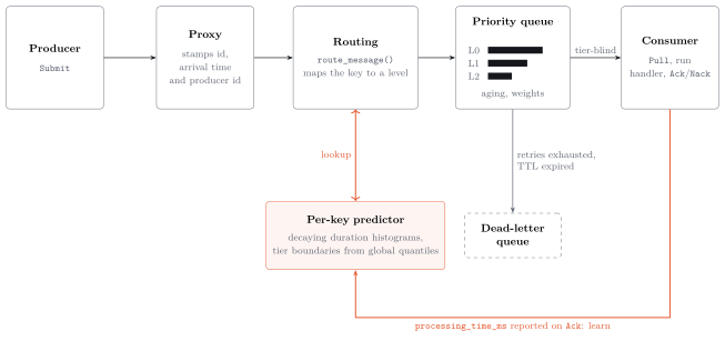
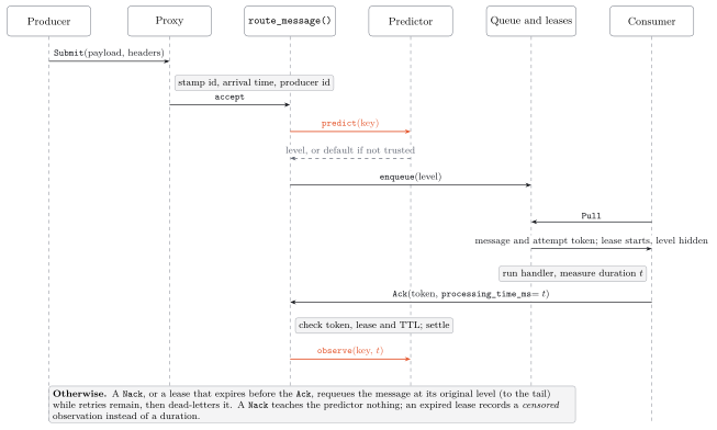
**Figure 1.** Overview of Harbinger. Messages flow left to right. The orange path is the learning loop: the routing function looks up a message’s key in the per-key predictor, and each acknowledgement reports the handler’s duration back to it. An illustration of the design, not a measurement.

Figure 2 follows one message through every exchange, in order. A producer’s Submit reaches the proxy, which adds the identifier, the arrival time and the producer’s identity and passes the message to the routing function. The routing function asks the predictor for the key’s level and receives either that level or, when the history is not trustworthy, the default. It then places the message in the queue. Nothing about the level is visible from there on: a consumer’s Pull returns the message with an attempt token, and the lease that bounds the delivery starts at that moment. The consumer runs its handler, measures how long it took, and reports that duration with its Ack. The broker checks the token, the lease and the message’s time to live, settles the delivery, and only then tells the predictor the duration, which is why a late or replayed acknowledgement teaches nothing. The failure paths are summarised under the figure: a Nack, or a lease that expires first, puts the message back at the tail of its original level until its retries run out, and an expired lease leaves a censored observation in place of a duration.

**Figure 2.** The exchanges for one message, in order. Black arrows are the ordinary delivery path, dashed arrows are returns, and the orange arrows are the two calls that connect the broker to the predictor: a lookup when the message arrives and an update when its acknowledgement is accepted.

The remaining subsections take the pieces in turn: the delivery core that exists with or without prediction, the choice of statistics over a learned model, the predictor and the checks that decide when to trust it, and then the optional features, each of which was added in response to a specific weakness that an experiment exposed. Each subsection says what the feature is, how it is built and what we saw when we measured it, and Table 2 at the end collects the results.

3.2 The delivery core

The first stage was an ordinary broker with no prediction at all. It has a fixed number of priority levels, an optional aging thread that promotes messages that have waited too long, retries on Nack, a dead-letter queue for messages that exhaust their retries or expire, and per-delivery attempt tokens and leases, so that a crashed consumer’s message is recovered while a stale acknowledgement cannot settle a newer delivery. Delivery is at-least-once for as long as the process runs, and all state is in memory. Static routing, in which every message gets the same default level, is what this stage gives and what the broker still does by default. It is also the baseline against which every later feature is measured.

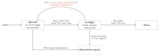
Figure 3 shows the delivery states that this stage defines. A message is queued until a Pull selects it, and it is then in flight, owned by one consumer under one attempt token. An acknowledgement within the lease completes it; a Nack or an expired lease returns it to the tail of its original level while retries remain; and exhausting its retries, or the expiry of its time to live, sends it to the dead-letter queue. The state machine is the same with or without prediction, which is what lets the predictor be added without changing delivery semantics.

**Figure 3.** Delivery states of a message. The orange arrow is the retry path; its destination is the message’s original level, which under predictive routing is the level the predictor chose.

3.3 Statistics instead of a model

The second stage was meant to add a learned classifier. We first planned a separate service fed with features captured at ingress and with durations persisted by the broker, and we built that plumbing: a bounded, versioned capture of ingress features and a bounded on-disk feedback log, both optional and neither able to change delivery. We then used it to compare eight online learners, including River regressors and trees (Montiel et al. 2021), against simple statistics, replaying the recorded workloads with the delay that real feedback has. None of the eight passed every frozen quality criterion. The rule was strict, requiring a model to be no worse than both arithmetic baselines on both metrics in every cell with no tolerance for noise, and the workload offered little for a richer model to exploit, because its only feature was a three-valued category and a per-key average is then close to the best possible predictor. We read the result narrowly. It did not show that learning cannot help, but it removed any reason to prefer a model, so we chose the simplest option. The predictor is an ordinary lookup, compiled into the broker, with no model to train or serve, and the Python tooling that produced the comparison stays offline.

3.4 Per-key duration prediction

A message’s key is the identifier the broker assigned to its producer, optionally joined to a job-type header that the producer chooses to send. Scoping the header by producer means that a producer can only mislabel its own work and cannot borrow another producer’s fast history to jump the queue. The broker keeps, for every key, a histogram of handler durations whose older observations decay, and one histogram over every key. Write $x_{k,1},\dots,x_{k,n_k}$ for the successful handler durations observed so far for key $k$ , in the order they were acknowledged, and $H_k$ for the key’s histogram over a fixed set of geometric duration bins $b$ . With a decay factor $d<1$ , each observation’s weight shrinks by $d$ every time a newer one arrives,

(1)

\begin{equation} H_k(b) \;=\; \sum_{i=1}^{n_k} d^{\,n_k-i}\,\mathbf{1}\!\left[x_{k,i}\in b\right], \qquad \hat{x}_k \;=\; Q_{1/2}(H_k), \end{equation}

where

Q_q(\cdot)

is the

q

-quantile of a histogram and the median

\hat{x}_k

is the key’s expected duration. After

h=\ln(1/2)/\ln d

new observations an old regime carries half the weight, which is how quickly the predictor forgets (about 138 observations for

d=0.995

). A successful, first-time duration reported on an acknowledgement is added to the message’s key; failures, replays and late settlements are not.

At ingress the broker maps the expected duration to a level using boundaries that come from the pooled histogram $G$ . With $L$ levels, its quantiles supply the boundaries, and the level is the number of boundaries that the estimate has reached,

(2)

\begin{equation} \beta_j \;=\; Q_{j/L}(G),\quad j=1,\dots,L-1, \qquad \ell(k) \;=\; \bigl|\{\,j : \beta_j \le \hat{x}_k\,\}\bigr|, \end{equation}

so that level

0

, the highest priority, holds the shortest expected jobs and the levels adapt to the workload instead of being set by hand. The lookup costs about a hundred nanoseconds in isolation and about 2.7 microseconds on average inside the running broker.

Figure 4 shows how the pieces fit on a concrete example. The top panel is the pooled histogram of every key, and its tertiles, shown by the dashed lines, are the two boundaries that divide three levels. Below it are four keys. A key whose handlers take a few milliseconds has its median to the left of the first boundary and is routed to the highest-priority level, one whose handlers take tens to hundreds of milliseconds falls in the middle, and one that takes seconds goes to the lowest. The last key is the case the next subsection is about.

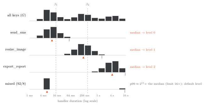
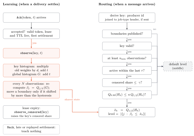
**Figure 4.** An illustration of how a key’s history becomes a level. Bars are decayed duration histograms on a logarithmic axis; the orange triangle marks each key’s median and the short bar its ninety-ninth percentile. The key shapes are made up, and the boundaries and levels are computed from them by Equation (1), Equation (2).

Figure 5 lays out the two paths through the predictor. The learning path, at the left, accepts only a settled delivery: the key’s histogram and the global histogram both grow, and the boundaries are recomputed periodically and move only when they have shifted by more than a small margin, so that a single unusual job cannot reshuffle the levels. The routing path, at the right, is a short sequence of questions, each of which can send the message to the default level, and only a message that passes all of them is routed by its estimate.

**Figure 5.** Inside the predictor. Left: what happens when a delivery settles. Right: how a level is chosen when a message arrives. Orange boxes touch learned state, and the dashed box is where every failed check lands.

The predictor can run in two modes. In shadow mode it records what it would have done but routes statically, which isolates the cost of prediction from its effect; in predictive mode it routes by its estimate. The first experiments (Section 5) passed on a production-style job queue but not on the Azure trace simulation, where no load passed its gate, so predictive routing stayed an opt-in.

3.5 Deciding when to trust an estimate

A predictor that routes on its own estimate has to know when not to trust it, and the routing path in Figure 5 is mostly this. Four conditions must hold, besides the technical ones that the boundaries have been published and that the key is valid. The key must have at least $n_{\min}$ observations; it must have been active within the last $\tau$ , which is thirty minutes; its tail must be close to its median; and the decayed share $c_k$ of its deliveries that overran their lease must be small,

(3)

\begin{equation} n_k \ge n_{\min}, \qquad t - t_k \le \tau, \qquad Q_{0.99}(H_k) \le \kappa\,Q_{1/2}(H_k), \qquad c_k \le \gamma, \end{equation}

with

\kappa=16

and

\gamma=5\%

. A message that fails any of them takes the default (middle) level

\ell_0

, and only one that passes all of them is routed by Equation (2). Time-based decay, eviction and the hysteresis that stops boundaries from jittering are omitted from the equations for clarity.

The tail check looks at the ninety-ninth percentile rather than the ninetieth, and the reason is the last key in Figure 4. Ninety-two percent of its jobs are fast, so its median would put it in the top level, but eight percent take thousands of times longer, and routing it by its median would let those jobs delay everything behind them. A test showed that a key like this looks unremarkable at the ninetieth percentile and was routed to a fast level, which is exactly the costly mistake the literature warns about (Dell’Amico et al. 2014). Its ninety-ninth percentile is far above sixteen times its median, so it takes the default level instead. A delivery that overran its lease yields no duration, so it is recorded as censored, and a key with many censored deliveries also falls back; dropping them would have made a key whose handlers hang look fast. Memory is bounded, with a fixed number of keys spread over sharded locks.

The trace simulation also exposed a defect in the staleness check, which we fixed. Staleness was measured from a key’s last completed job, so during a backlog lasting hours a key whose jobs were stuck in the queue completed none, and its new messages were judged stale and sent to the default level. The predictor switched itself off for exactly the keys caught in the backlog, and in an exploratory run a third to a half of the predictions made during backlogs were stale verdicts, against well under one percent otherwise. Activity now includes a prediction made while the key was still fresh, so keys that are waiting in a backlog stay predicted, though a stale key is revived only by new evidence.

Table 1 lists every parameter that shapes routing, with the value used in every experiment in this paper. The operator sets none of them per endpoint, but they are not free of judgement: we chose them by reasoning about the workloads, the 99th-percentile spread check was chosen after a test showed the 90th percentile missed bimodal keys, and the staleness rule changed after the Azure simulation (below). We varied them only afterwards, one at a time and in the simulator: the weighted design’s gate was robust to every one, the strict-priority design’s was not, and the aging threshold mattered most (Section 5.5). The values in the table are the ones used throughout.

**Table 1.** The predictor’s and aging’s parameters, as used in every experiment. None is set per endpoint. The values were fixed by judgement before any sweep (Section 5.5).
Parameter	Value	Role
Levels $L$ ; default level $\ell_0$	3; the middle level	number of priority levels; where untrusted keys go
Minimum observations $n_{\min}$	20	a key is predicted only after this many successful durations
Spread check $\kappa$	16 at the 99th percentile	a key whose $Q_{0.99}$ exceeds $\kappa$ times its median takes the default level
Censored share $\gamma$	5%	a key with more lease or TTL overruns than this takes the default level
Key decay $d$	0.995	per-observation retention; half-life about 138 observations
Idle half-life	10 min	wall-clock decay of a key’s history across idle gaps
Staleness $\tau$	30 min	a key with no activity this long is not predicted
Pooled decay	0.9999	retention of the histogram that sets level boundaries
Boundary refresh; minimum pooled samples	every 256 observations; 100	how often boundaries are recomputed, and when the first are published
Aging threshold and interval	5 s; 0.5 s	a message waiting longer than the threshold moves up one level
Level weights (opt-in)	8, 3, 1	worker-time shares under the weighted design

3.6 Aging

Reordering by expected duration invites starvation, since a long job can be passed over indefinitely by a stream of short ones, so the broker has an aging mechanism. A background thread runs at a fixed interval (half a second), visits the levels from the lowest upward, and moves any message that has waited longer than a threshold (five seconds by default) to the back of the next level up, resetting its wait. A message that keeps waiting is promoted again after another threshold, so a message reaches the top level after at most the threshold times the number of levels it must climb, and no message can be left at a low level indefinitely.

This works well when backlogs last seconds, and it is the right behaviour for a queue in which waiting is the exception. It does not work when they last minutes or hours. Then almost every waiting message has waited longer than the threshold, so promotion carries each one upward as soon as it is eligible, and the top level fills with work that the predictor had placed lower. The ordering the predictor produced is erased, because all levels converge on one first-in-first-out queue. This is the likely reason the Azure simulation did not pass, since the oracle, which has perfect predictions, did no better; we did not switch aging off on Azure, and in the simulator a thirty-second threshold still cut gate A’s mean latency by only 3.4%. It is also why the opt-in described next exists. Figure 7 in the next subsection shows the effect in a small model. The effect is also measured: with aging switched off, predictive routing’s mean latency on the production flow fell a further 37.4%, and on Huawei Cloud through the real broker it passed the gate that it fails with the default aging (Section 5.3). The price is the protection, since without aging a long job can be passed over indefinitely, which runs of five and twenty-five minutes are too short to show.

3.7 Weights and pausing aging

For that regime we added, as an option, a scheme in which the levels share worker time by weights instead of strict priority. Each level $\ell$ has a weight $w_\ell$ and a virtual clock $v_\ell$ that starts at zero. A pull serves the non-empty level with the smallest clock and charges that level the message’s expected cost $\hat{c}$ divided by its weight,

(4)

\begin{equation} \ell^{\star} \;=\; \arg\min_{\ell\,:\,\text{level }\ell\text{ non-empty}} v_\ell, \qquad v_{\ell^{\star}} \;\leftarrow\; v_{\ell^{\star}} + \frac{\hat{c}}{w_{\ell^{\star}}}, \end{equation}

so that, while every level has work, level

\ell

receives a fraction

w_\ell/\sum_{j} w_j

of worker time: two thirds, a quarter and a twelfth for the weights

(8,3,1)

that we use. An empty level cannot save credit for later. 6 applies the rule to a backlog in which every level always has work.

**Figure 6.** The weighted-share rule applied to a backlog in which all three levels always have work and every message costs the same. The top strip shows the first 48 pulls in the order the rule serves them; the bars show each level’s share of pulls against its ideal share $w_\ell/\sum_j w_j$ (orange mark). A computed illustration of the rule, not a measurement.

Weights alone do not fix the collapse, because plain aging would still refill the top level. Pausing aging therefore skips the promotion of a message from level $\ell$ to $\ell-1$ for as long as level $\ell-1$ is behind, meaning that it still holds promoted messages and its oldest message has waited at least the aging threshold, and a pass promotes at most one message per level. The first implementation of this rule was wrong, and we corrected it before pre-registering the experiment. Figure 7 shows what the two promotion rules do under sustained overload in a toy model that applies the rules as described. Under strict priority with plain aging, about half of the top level is soon promoted work, and the wait of jobs the predictor put in the top level climbs steadily. Under weights with pausing aging, promoted work stays a small fraction and their wait levels off, but the lowest level’s backlog grows much larger, and that is the price: the longer jobs wait longer, which is the same trade that the production-flow results show.

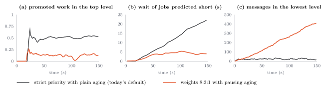
**Figure 7.** A toy model of the two promotion rules under sustained overload: arrivals at 120% of capacity for 150 seconds, with half of the jobs predicted short, three tenths medium and two tenths long, a five-second aging threshold, and equal service times. (a) The share of the top level that is promoted work. (b) The mean wait of jobs predicted short. (c) The number of messages in the lowest level. A computed illustration of the rules, not a measurement; the weighted design wins on (a) and (b) and pays on (c).

The measured effect was as the toy suggests but with a cost. On the Azure trace the weighted design cut mean latency against FIFO by 14.6%, 23.7% and 27.3% at loads of 0.5, 0.8 and 0.95, and by 13.9% to 25.0% against the default aging, but its gate passed only at load 0.8. On the production flow it cut mean latency by 41.9% against predictive routing with default aging, but raised all-message P99 by 12%, over its ten-percent guardrail, so that gate failed too. Replicated on AWS, with the same frozen configuration, the gate again did not pass: the mean was 38.4% lower, and all-message P99 was 10.0% higher, with an interval whose upper end, 10.7%, is still over the guardrail. The weights and the pausing rule therefore stay opt-in. The stronger evidence is later: replayed through the real broker, the weighted design passed its gate at loads 0.8 and 0.95 on both the Azure and the Huawei trace (5.2).

3.8 Size-binned keys

A per-key median ignores the fact that some jobs cost what their input costs. We measured how much that matters on self-generated data with real handlers, and asked whether a richer model was needed to capture it. It was not. A per-key median was off by a typical factor of 1.9 and placed jobs in the correct level 68% of the time, while appending the logarithm of the input size to the key brought the factor down to 1.2 and the accuracy up to 93%, and a gradient-boosted model over every feature did no better at 93%. So we added the bin to the key, not a model.

The bin is an optional $\log_2$ size, read from the payload length or from a numeric header and appended to the key. A bin that has not yet seen enough jobs borrows its un-binned parent’s estimate, never another key’s, and each job teaches both the bin and its parent, so a new bin is not cold for long. Under load the result was weaker than the measurement suggested. The bins improved the predictor’s accuracy, but mean latency changed by only $+$ 0.7% [ $+$ 0.5, $+$ 0.9] against job-type keys, short of the pre-registered bar (on AWS, $-$ 1.5% [ $-$ 4.5, $+$ 0.4], which also missed it), and one job type whose cost does not follow its size did 8.7% worse. They remain an opt-in.

3.9 Operating the predictor

Alongside these features we built the operational pieces that make the predictor safe to run. Predictor state is saved to atomic, versioned snapshots with a rollback copy, so that a restart does not start cold and a corrupt file is refused instead of trusted. Counters record why each message fell back, and drift signals, namely rolling agreement between predicted and actual level and a running average of the log error, are informational and never change the routing. A standalone configuration file selects the mode and has a one-line switch back to static routing. None of these changes the order in which messages are delivered. They are what let an operator turn prediction on in shadow mode, look at what it would have done, and turn it off again.

3.10 Summary of the opt-in features

Table 2 collects the optional features, why each was added, and what the experiments showed. The pattern is worth stating plainly. Each feature was added in response to a specific weakness, each was tested against a criterion set before the run, and none of them passed every gate it faced, which is why the broker’s defaults are still static priority with no prediction.

**Table 2.** Opt-in features, why each was added and what the experiments showed. The default for every row is off.
Feature	Added because	What the experiments showed
Predictive routing	static priorities need a person who knows each job’s cost	passed on the production flow and on AWS; failed its gate in every cell of the Azure and Huawei replays with default aging
Size-binned keys	per-key medians ignore input size	more accurate predictions, but no reliable latency gain under load; one job type got worse
Weights and pausing aging	default aging collapses the levels in long backlogs	passed its gate at loads 0.8 and 0.95 on both replayed serverless traces and cut mean latency on RabbitMQ; all-message P99 rose in the production flow
Ingress features and persistent feedback	to compare candidate learners offline	enabled the comparison; no learner beat per-key statistics

4 Evaluation method

A scheduling claim is easy to overstate, so we fixed what would count as success before running the experiments that support it. Each experiment has a configuration and a set of pass criteria committed to the repository before its first registered run, and the commit that froze them is recorded alongside the results. A criterion compares an arm against a baseline as a paired difference, per seed or per time window, with a bootstrap 95% interval, and a gate passes only when every primary criterion does. Concretely, for a metric $M$ such as mean latency, the unit of pairing is a seed (or, in a simulation, a time window) $u$ , and a relative-delta criterion is the average of the paired differences,

(5)

\begin{equation} \Delta \;=\; \frac{1}{|U|}\sum_{u\in U}\frac{M_u^{\text{arm}}-M_u^{\text{FIFO}}}{M_u^{\text{FIFO}}}, \end{equation}

with its interval taken by resampling the units; a ratio criterion averages

M_u^{\text{arm}}/M_u^{\text{FIFO}}

in the same way. Slowdown is a job’s latency divided by its own service time. The primary criteria concern mean latency and the median latency of short jobs. All-message P99 and the longest wait of a long job are guardrails, which a design must not break, and are not goals. We should be honest about the limits of this discipline: the budgets for the first experiment were chosen after we had seen data from an earlier offline study, so they are not independent of it. Deviations from the pre-registrations are listed here. Every frozen configuration is unchanged since the commit that froze it. One amendment was made during the AWS runs: the single-host replication moved to its own instance when the vCPU quota rose, before its first run and with only message counts read. The thirty-minute run was registered as descriptive, with no gate. The first trace simulation on Azure, before the weighted design, used older simulator rules, and a staleness defect found there was fixed before the later experiments; the common-rules runs on Azure use the converted trace and time-based windows, so their figures differ slightly. The DAS2 diagnosis and the quiet-machine re-run were run afterwards and are not pre-registered, and the re-run keeps the frozen configurations and analysis. The four experiments of 14 and 15 October (the baselines and aging isolation, the parameter sweep, the trace replay and the aging-off replay) were pre-registered too. In the replay, Azure runs the three gate arms at loads 0.5 and 0.95 and all five arms at 0.8, once per cell, because its cells take hours; the two research-cluster logs were dropped from it, because their time scales would put the broker’s aging constants at one to seventeen milliseconds, where scheduler jitter is comparable; and two Huawei cells lost the broker and were re-run once, as the pre-registration allows, with both attempts kept. The aging-off replay ran on two smaller hosts and so carries its own FIFO and predictive arms. Two bugs in the replay analysis script were fixed after its first use on the aging-off run and before any replay result was read as final; neither touches a gate number, and both have tests. The sweep’s second stage, a confirmation of its flipping variants on the real broker, was never run (6).

The arms follow the questions the experiments ask. FIFO is the default behaviour of most queues. Two static-priority baselines stand for what an operator would do by hand: one set by someone who knows each job type’s cost, and one set badly but plausibly, in which an expensive and a cheap job share a level. Shadow mode measures the cost of prediction without its effect, and predictive mode routes by prediction, with or without job-type labels. An oracle that ranks messages by their true planned cost shows how much room a perfect predictor would leave. We treat the oracle as a reference rather than an optimum, since it ranks by fixed terciles and costs are only approximate under contention.

The main workload is a synthetic production flow (3) that we designed to look like the background work of an online shop. Five services produce nine job types, from cheap jobs such as stock reservation to long report exports, and the handlers do real CPU work through the real producer and consumer clients. Load follows a steady phase at about sixty percent utilisation, a flash-sale overload at about one hundred twenty-five percent, a recovery, and a mid-run change in job costs, with about thirty-five thousand messages per run and five seeds. We ran it locally, on a laptop with turbo disabled (Section 5 gives the conditions), then on AWS with the broker and the clients on separate hosts (c8i.xlarge and c8i.2xlarge instances in one placement group), and replicated the original single-host run on a second instance of the larger type. The same workload then ran against RabbitMQ with FIFO, with static priorities, and with Harbinger’s predictor acting as a sidecar that sets the priorities, and against Redis with FIFO, with the same producers, handlers, workers, arrivals and seeds so that only the broker and its policy change. A thirty-minute run, in two repetitions, tests whether the benefit survives long backlogs. Two further frozen production-flow experiments test the design’s optional features: one compares weights and pausing aging with predictive routing under the default aging, and one tests keys split by input size. A third, on ten seeds on AWS, compares predictive routing with a queue per job type served in equal shares of worker time with no prediction, with the mean and 75th-percentile summaries, and with each of four predictor components removed, and it switches aging off to isolate its effect. A one-at-a-time sweep of the predictor’s and aging’s parameters ran in the simulator. An offline comparison of eight online learners against per-key statistics, on recorded workloads, decided whether a model was needed at all.

**Table 3.** The wall-clock experiments. The first three run the same synthetic production flow (five services, nine job types, about thirty-five thousand messages in a five-minute run, 4 workers); E2 runs it for thirty minutes and E4 uses empty handlers. Arms are the policies compared in each run.
Experiment	Hardware	Run	Arms	Runs
Local re-run (v2)	Laptop, 8 cores, turbo off; broker in process	300 s	7	5 seeds, 35 runs
AWS replication (E1)	c8i.2xlarge (8 vCPU); broker in process	300 s	7	5 seeds, 35 runs
Brokers (E3)	c8i.2xlarge clients, c8i.xlarge broker	300 s	8	5 seeds, 40 runs
Long backlog (E2)	Same pair of hosts	30 min	4	2 repetitions, 8 runs
Broker cost (E4)	Same pair of hosts	30 s per rate	3 brokers	4 offered rates, 5 repetitions

Real traces test what a synthetic workload cannot: whether keys recur and how heavy the tails are in practice. A discrete-event simulator replays the Azure Functions 2021 trace (Zhang et al. 2021) (its earlier characterisation is Shahrad et al. (2020)), the Huawei Cloud public request traces (the 2025 release, described by Joosen et al. (2025); the earlier 2023 release is described by Joosen et al. (2023)) and two Parallel Workloads Archive logs (Feitelson et al. 2014) (4) at offered loads of 0.5, 0.8 and 0.95, using the same predictor code as the broker and a common trace format (Section 6 reports how well the simulator reproduces the broker). Arrivals are reconstructed where a trace lacks them, and one of the traces records completion times instead of arrival times, which we discuss with the limitations. Two gates are defined for each trace. Gate A asks whether predictive routing, as built and with the default aging, beats FIFO. Gate B asks the same of the design with weights and pausing aging. The numbers in the tables and the headline results are generated from the committed result files by a script in the paper’s repository. A few figures quoted in the text are typed by hand from the repository’s reports and were checked against them: the original local run’s effect sizes, the percentages of the DAS2 diagnosis, the counts of replay cells, and some one-off ratios. The guardrails are judged on the upper end of their intervals.

The simulator is not the broker, and the production-flow check found that it overstated a gain (Section 6), so the Azure and Huawei traces were also replayed through the real broker on AWS. A producer submits each message at its scheduled arrival, compressed so that the mean offered load over the evaluation half is the target, and 64 consumers stand in for the workers. Their handlers do no real work: each simply waits for the job’s recorded duration and then acknowledges, so the queueing, ordering and aging are real but the CPU contention that real handlers cause is absent. Azure runs at a time scale of 4.5, with the broker’s aging, staleness and forgetting constants divided by the same factor, so that its seven days fit in hours; Huawei runs at real speed. The predictor is warmed on the history half offline, through the broker’s own code, and handed to the broker as a snapshot. Trace keys travel as short labels, because the broker rejects job keys over 128 bytes, which Azure’s are, and an over-long key is silently left unpredicted. Latency is measured from a message’s scheduled arrival, and a run counts only if every message completes, with no dead-lettered message or lost lease, and producer lateness stays under 10 ms. The evaluation half is cut into 28 windows of equal time, and the primary interval is a moving-block bootstrap over the paired per-window changes with blocks of four windows, because adjacent windows share a backlog; the seven-window interval of the simulation is reported beside it. Huawei cells run three times and are pooled, and a gate cell whose repeats disagree is reported as unstable and does not count as a pass; none was. A run that fails these rules is kept and repeated once.

Two mean-latency figures appear for the traces, and they differ. The gated figure, in Table 16, Figure 12 and wherever the text says a gate arm cut mean latency, is the average of the per-window paired changes of Equation (5), so each window counts equally however much work it holds. The whole-run figure, in Table 13 and in the seconds quoted for Huawei, compares the mean over every job of the evaluation half, so windows with many jobs or long backlogs dominate it. The gap can be large: for the weighted design at load 0.8 the window-averaged change is $-$ 15.3% on Azure and $-$ 37.0% on Huawei, and the whole-run change is $-$ 7.9% and $-$ 90.4%. On Azure the last day holds most of the work, and the backlog there dominates the whole-run figure. Both are descriptive of the same runs; the gates use the window average.

**Table 4.** The four traces. Each is split by time into a history half, which warms the predictor, and an evaluation half, replayed on 64 workers at offered loads 0.5, 0.8 and 0.95, simulated for all four traces (seven windows) and, for Azure and Huawei, also replayed through the real broker (28 windows). Job and key counts are those of the converted files (the preregistrations and the converter report them).
Trace	Content	Jobs	Keys	Span	Key	Arrival
Azure Functions 2021	serverless invocations	1,980,951	424	14 days	app and function	end time minus duration
Huawei Cloud 2025	serverless requests, one region	3,443,079	491	1 day	function	completion minus frontend cost
LPC-EGEE 2004	grid cluster jobs	214,322	219	4 months	user and queue	recorded submit time
DAS2-fs2 2003	research-cluster jobs	64,660	2,516	6 months	user and executable	recorded submit time

The experiments were not independent of each other, because later designs were built in response to earlier failures. 5 says, for each, what had been seen before it was frozen, so that a reader can tell which results are tests of a fixed design and which are not. In short, the Azure trace motivated the staleness fix and the weighted design, so its weighted results are in-sample for the design; Huawei Cloud, the two research logs and the AWS runs were first run under rules that were already frozen.

**Table 5.** What informed each experiment before its configuration was frozen. “Out of sample” means that the design and parameters under test were fixed before the first scheduling run on that data.
Experiment	Frozen	What had been seen; status
Production flow, local	5 Oct	budgets chosen after earlier offline data and two FIFO-only load pilots, so not blind; no predictive arm had run
Azure 2021 simulation	5 Oct	first trace; predictive routing failed at every load, which exposed the staleness defect and the aging collapse
Weights and pausing aging	8 Oct	designed in response to the Azure result, so Azure is in-sample for the design; frozen before its first registered run on Azure and on the production flow
Size-binned keys	8 Oct	motivated by an earlier offline study of input size; tested under load for the first time here
Huawei Cloud 2025 simulation	11 Oct	both designs fixed before any scheduling arm ran on this trace; out of sample, but its conversion rules were checked on the data
Azure under common rules	11 Oct	same trace as the design above, so in-sample
LPC-EGEE and DAS2-fs2	12 Oct	rules unchanged from the Huawei run; out of sample
AWS replication and brokers	12 Oct	frozen after an AWS debug pass; new hardware, but the same workload, so out of sample for hardware only
AWS reruns of aging and size bins	14 Oct	the frozen configurations of 8 Oct, unchanged, on new hardware; the local results were known, so these replicate and do not test a new design
Simulator validation	14 Oct	replays the measured production-flow runs, which were already published, through a simulator that had never run on them; its effect-size criterion failed (Section 6)
Baselines and aging isolation	15 Oct	chosen after the aging and sidecar results were known; the aging-off arm tests an explanation we had already formed, so its result tests that explanation and was not a discovery
Parameter sweep, simulator	15 Oct	grid fixed before any variant ran; Azure’s results were known, so Azure is in-sample for the design being varied
Trace replay	15 Oct	frozen after the simulator verdicts, the sweep and the baselines were seen; loads and arms were chosen from the simulator’s results (Azure’s gate arms at 0.5 and 0.95 only), but no replay cell had been read
Aging-off replay	15 Oct	chosen after the sweep and the baselines pointed at aging; frozen before any replay cell was read
DAS2 diagnosis, quiet-machine re-run	after	run after the results were seen; not pre-registered

5 Results

We begin with a map of the claims and what stands behind each (6); the rest of the section follows it. A claim is marked supported only where its experiment met the bar registered for it.

**Table 6.** Claims, the experiment behind each, whether the design under test was fixed before that experiment (Table 5), and the verdict. The simulator verdicts are for the experiments in which it stood in for the broker.
Claim	Experiment and setting	Fixed beforehand?	Verdict
Predictive routing beats FIFO and a hand-tuned map on a mixed job queue	production flow, five seeds, real handlers; local and AWS	budgets set after earlier offline data; AWS is a replication	Supported: mean latency cut by 25.6% locally and 30.8% on AWS
The gain does not depend on our broker	same workload on RabbitMQ and Redis; sidecar; AWS	yes, for the hardware only	Supported; our own FIFO is 11.0% slower than RabbitMQ’s
It improves the all-message tail	P99 against FIFO, production flow	yes	Not claimed: P99 stays within 1.03 $\times$ of FIFO’s, and mid-cost jobs wait longer
Default aging limits the gain under long backlogs	aging off: production flow (ten seeds) and Huawei, real broker	chosen after the aging result was known	Supported on those two; untested on Azure
Weights and pausing aging pass on serverless traces	Azure and Huawei replays, real broker, sleeping handlers	Azure in-sample for the design; Huawei out of sample	Partly: 4 of 6 cells, none at load 0.5; Azure at 0.8 by 0.3 points on one run
Predictive routing as built passes on those traces	same replays	fixed before the runs	Not supported: 0 of 6 cells
Prediction is needed for the gain	queue per job type (production flow); static map from history (Huawei)	chosen after the main results were known	Not supported: the per-type queue was 42.1% lower in mean latency, and a static map matched or beat the predictor on Huawei
It helps on HPC logs, where keys recur rarely or predict poorly	LPC-EGEE and DAS2-fs2, simulated	fixed before the runs	Not supported: no gain on LPC-EGEE, harm on DAS2-fs2
Size-binned keys improve latency	production flow, local and AWS	fixed before the runs	Not supported: missed the bar twice
The simulator reproduces the broker	production flow; Azure and Huawei replays	fixed before the runs	Mixed: effect-size bar failed on the production flow (overstated by about 41%); within 1.3 points on the replays

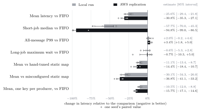
We begin where the design was meant to work, a shared job queue whose job types differ in cost. In the production-flow benchmark, predictive routing passed its pre-registered gate (Figure 8; criteria and bars in Table 14, Appendix A). Against FIFO it reduced mean latency by 25.6% and the median latency of short jobs by 57.7%, while all-message P99 stayed within 1.02 $\times$ of FIFO’s and no work was lost. It also did better than what an operator would have done. Compared with a hand-tuned static map it was 11.1% lower in mean latency, and compared with the plausible but misconfigured map it was 30.1% lower, a map that was itself slower than FIFO. Even without job-type labels, with one key per producer, it reduced mean latency by 10.5%, about two fifths of the benefit of labelling. The replication on separate AWS hardware reproduced every verdict, with a mean reduction of 30.8% and a short-job median reduction of 94.8%. The predictor also sat close to a perfect-cost reference: the oracle arm cut mean latency by 25.1% locally, against 25.6% for the predictor, and by 33.1% on AWS, against 30.8%.

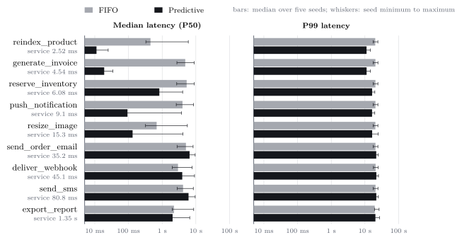
**Figure 8.** Production-flow benchmark: change in latency against each comparison, in a local quiet-machine re-run and its replication on AWS. Bars are paired point estimates over five seeds, whiskers are 95% bootstrap intervals and each hollow dot is one seed’s own paired value; for P99 and maximum wait the bar is the ratio minus one. Every criterion met its pre-registered bar in both runs (Table 14).

The gain is not shared evenly, and the figure by job class shows who pays (Figure 9). Ordered by their median service time, the cheap classes (reindex_product, generate_invoice) went from waiting hundreds of milliseconds to seconds at the median to tens of milliseconds, and their P99 fell by about 45%. The classes in the middle, whose handlers take tens of milliseconds, did worse at the median than under FIFO: send_sms, send_order_email and deliver_webhook each waited 29% to 45% longer at P50. That is the price of putting short work first, and it is paid by jobs that are only moderately long. export_report, the one genuinely long class, was close to unchanged. Across five seeds the whiskers are wide for several mid-cost classes, so we read the direction of these effects and not their size.

**Figure 9.** Per-class latency in the AWS production flow, FIFO beside predictive routing, with classes ordered by median service time (cheapest first). The axis is logarithmic. Predictive routing cuts the median of the cheap classes by one to two orders of magnitude and their P99 by about half, raises the median of the three mid-cost classes, and leaves the one long class about where it was.

The mean over a whole run is dominated by the flash sale, where FIFO’s mean latency is tens of seconds, so Table 7 breaks it down by phase. The gain is not confined to overload. In the steady phase, at about sixty percent load and with waits of tens of milliseconds, predictive routing cut mean latency by 20% on AWS and 28% locally, and in every phase and for every seed it was below FIFO. The largest absolute savings, in seconds, come from the flash sale and the recovery that follows it. These rows are descriptive and are not separate pre-registered criteria.

**Table 7.** Mean latency by workload phase in the production flow: FIFO’s mean (median over five seeds, ms), and the change in mean latency under predictive routing (mean of the per-seed paired changes, with the smallest and largest seed in brackets). Descriptive; the phases are not separate pre-registered criteria.
	Local run			AWS replication
2-4(lr)5-7 Phase	FIFO	Change	Seed range	FIFO	Change	Seed range
Steady (about 60% load)	92	$-$ 28%	[ $-$ 31%, $-$ 26%]	48	$-$ 20%	[ $-$ 27%, $-$ 13%]
Ramp	744	$-$ 47%	[ $-$ 49%, $-$ 43%]	243	$-$ 48%	[ $-$ 54%, $-$ 40%]
Flash sale (about 125% load)	16,598	$-$ 31%	[ $-$ 36%, $-$ 27%]	12,428	$-$ 34%	[ $-$ 42%, $-$ 29%]
Recovery	22,613	$-$ 17%	[ $-$ 20%, $-$ 14%]	13,051	$-$ 23%	[ $-$ 32%, $-$ 17%]
After the cost shift	14,367	$-$ 29%	[ $-$ 38%, $-$ 17%]	651	$-$ 53%	[ $-$ 62%, $-$ 40%]

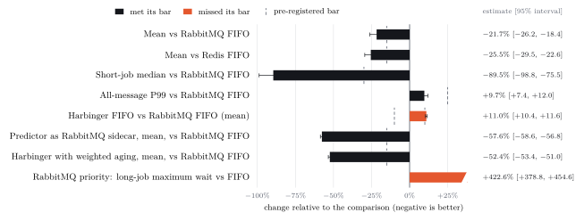
The result does not depend on the broker being ours. Run against RabbitMQ and Redis on the same workload (Figure 10, 15), Harbinger’s predictive arm reduced mean latency by 21.7% against RabbitMQ with FIFO and by 25.5% against Redis with FIFO, and the gate passed. The margin was smaller than we had predicted, partly because Harbinger’s own FIFO arm was 11.0% slower than RabbitMQ’s, just outside the pre-registered equivalence bar: the broker adds latency of its own under this load. The more telling result is what happens when the predictor leaves Harbinger behind. Running beside RabbitMQ as a sidecar that sets message priorities, it cut mean latency by 57.6%, well beyond what it achieved inside Harbinger. The likely reason is aging. RabbitMQ’s priorities never age, so short jobs stay ahead through the whole flash sale, while Harbinger’s default aging eventually lifts waiting long jobs back to the top. This experiment does not isolate it, but a later one does (Section 5.3): with aging switched off, predictive routing inside Harbinger cut mean latency by 57.6% against FIFO on the same workload, about the size of the sidecar’s gain, though against a different FIFO baseline and on different hosts, so the two are not compared by a test. With weights and pausing aging Harbinger cut it by 52.4% against RabbitMQ FIFO, at the price of an all-message P99 of 1.21 $\times$ RabbitMQ FIFO’s. The price of aging’s absence is the other way round: static priorities without aging made the longest wait of a long job 5.2 $\times$ that of FIFO. In a separate cost measurement with empty handlers, Harbinger delivered about 5,300 messages per second at its limit against 7,400 for RabbitMQ and 21,200 for Redis, so it is the slowest of the three (RabbitMQ ran with a prefetch of one, which also limits its throughput). At 5,000 messages per second offered it was already at its limit, and at 20,000 it fell behind in all five repetitions while RabbitMQ kept up in all five and Redis in three. This matters little against handlers that take milliseconds to seconds, but it does show up in the FIFO gap above.

**Figure 10.** Harbinger, RabbitMQ and Redis on the same flash-sale workload on AWS: change in latency against each broker’s FIFO arm, with the pre-registered bar marked. Bars are paired point estimates over five seeds and whiskers are 95% bootstrap intervals; ratios are drawn as ratio minus one, and the RabbitMQ-priority bar runs off the axis at $+$ 423%, and its pre-registered bar of $+$ 100% is also off the axis. Two criteria missed their bar: Harbinger’s own FIFO is slower than RabbitMQ’s, and RabbitMQ’s strict priority leaves long jobs waiting five times as long as under FIFO (15).

5.1 Why the mean falls and the tail does not

Before turning to long backlogs it is worth asking why the production flow behaves the way it does, because classical queueing theory gives a compact account of it. Take one server with Poisson arrivals and split the jobs into a short class and a long class, with arrival rates $\lambda_s,\lambda_l$ , service times $S_s,S_l$ and loads $\rho_s=\lambda_s\mathbb{E}[S_s]$ , $\rho_l=\lambda_l\mathbb{E}[S_l]$ , so that $\rho=\rho_s+\rho_l<1$ . Let $W_0=\tfrac12\sum_{c}\lambda_c\mathbb{E}[S_c^2]$ be the mean residual work seen by an arrival. Under FIFO, every job waits $W_{\text{FIFO}}=W_0/(1-\rho)$ . If instead the short class is served first, without preemption, Cobham’s formulas (Cobham 1954) give

(6)

\begin{equation} W_s \;=\; \frac{W_0}{1-\rho_s}, \qquad W_l \;=\; \frac{W_0}{(1-\rho_s)(1-\rho)} . \end{equation}

Dividing by

W_{\text{FIFO}}

shows that the size of each class’s change depends only on two loads,

(7)

\begin{equation} \frac{W_s}{W_{\text{FIFO}}} \;=\; \frac{1-\rho}{1-\rho_s}, \qquad \frac{W_l}{W_{\text{FIFO}}} \;=\; \frac{1}{1-\rho_s}, \end{equation}

and that reordering only moves waiting time from one class to the other:

\rho_s W_s+\rho_l W_l=\rho\,W_{\text{FIFO}}

, an instance of Kleinrock’s conservation law (Kleinrock 1965). The short class gains by a factor that grows as the load approaches one, while the long class loses by a factor of only

1/(1-\rho_s)

, which stays modest when long jobs carry most of the work. Averaged over all jobs, with

p=\lambda_s/(\lambda_s+\lambda_l)

the share of jobs that are short, the mean wait relative to FIFO is

(1-p\rho)/(1-\rho_s)

, which is below one exactly when

p\rho>\rho_s

, that is, when the short class’s share of the jobs exceeds its share of the work. That holds whenever the short class is shorter than average, so the mean always falls, and it falls more the more skewed the sizes are (Figure 11). The same equations also say why P99 does not improve. When more than one job in a hundred is long, the all-message 99th percentile is set by long jobs, and Equation (7) shows that their wait cannot fall: it rises by a factor of

1/(1-\rho_s)

. This is the shape of the production-flow results above, a large gain in mean and short-job median with all-message P99 within a few percent of FIFO’s.

**Figure 11.** Mean waiting time under non-preemptive priority relative to FIFO, from the closed forms above, for three mixes of short and long jobs. The short class gains more as load approaches one, the long class loses by a bounded factor, and the all-jobs mean always falls. This is an illustration of the model, not a measurement; the plotted points are tabulated in Table 18.

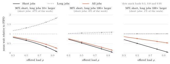
The model is an idealisation, and the experiments depart from it in three ways that the reader should keep in mind. It assumes one server, whereas the broker feeds several workers, and for several servers the analysis gives bounds rather than such a closed form (Scully et al. 2020). It assumes Poisson arrivals, whereas the flash sale is a burst. And it assumes perfect classification, whereas the predictor makes mistakes. It also describes waiting time, while the latencies we report add each job’s service time, which no ordering changes, so the measured reductions are smaller than the waiting-time ratios suggest. The model nevertheless sets a bound on what to expect from an ideal order, and we use it that way. On DAS2-fs2, where long jobs carry most of the work, an ideal order would have cost them only about a tenth more waiting at load 0.8, yet they waited several times longer. The excess cannot come from reordering as such. The oracle with the same scheduler improved every window there, so the likelier source is the predictor’s mistakes, which Equation (7) does not include.

5.2 Long backlogs and the traces

The benefit shrinks when backlogs last longer. In the thirty-minute run, with the broker on its own host, the reduction in mean latency fell to 6.1% and 7.4% in the two repetitions, short of the pre-registered bar. Three of the eight checks failed in all: the short-job median fell by 19.7% and 31.8%, so the first repetition missed its bar, and the mean after the mid-run cost shift fell by 14.7% and 23.1%, so the first repetition missed that bar by 0.3 points. P99 and the longest wait of a long job stayed level with FIFO, and the predictor still beat the hand-tuned map, by 2.2% and 3.1%. Outside overload the predictor still cut latency substantially; it was the six-minute flash sale, which pushed FIFO’s mean latency above a minute, and the long recovery after it, that dominated the overall mean. At those waits the default aging promotes nearly every message to the top level, so the order barely changes. This is the pattern the traces make explicit.

The traces show it at its clearest (Figure 12, 16). We replayed the Azure and Huawei traces through the real broker on AWS, with handlers that sleep for each job’s recorded duration; this isolates the queueing and leaves out the contention that real work would add. Predictive routing as built, with the default aging, failed its gate in all 6 cells. On Huawei it cut mean latency (window-averaged, Section 4) by 10.9% at load 0.8 and 8.4% at 0.95, short of the pre-registered 15%, and on Azure by no more than 2.2%. The oracle with the same aging failed too: it cut Huawei’s mean by 12.7% at load 0.8 and Azure’s by only 2.4%. The backlogs are long enough for aging to erase most of the order, and on Huawei Section 5.3 shows that it is aging and not the predictor: with aging switched off the same predictor passes. We did not run that test on Azure, where the oracle with the same aging also fails, which is consistent with aging but does not show it.

With weights and pausing aging the same predictor passed its gate at loads 0.8 and 0.95 on both traces and failed at 0.5, four of six cells, with reductions of 37.0% and 47.1% on Huawei and 15.3% and 17.2% on Azure. The cost fell where theory says it should. On Huawei at load 0.8 the whole-run mean latency fell from 17.9 s under FIFO to 1.7 s, and the median latency fell from 9.3 s to 65 ms, while long jobs waited a little longer (their longest wait stayed within 1.14 $\times$ of FIFO’s) and the all-message P99 stayed within 1.07 $\times$ . The failures at load 0.5 are a regime without much queueing, in which every policy is close to the service time. Azure’s gain is small in absolute terms and its load-0.8 cell passes by 0.3 points on a single run, so we read Azure’s gate B as a pass at the margin; the three Huawei repeats agreed on every cell. That the same weighted design works on two serverless providers, and that adding it over today’s aging is a further 33.4% reduction on Huawei and 14.2% on Azure at load 0.8, is consistent with the aging mechanism, and not the particular predictor, being the lever under sustained overload, although the weights change the scheduling as well as the aging, so this does not isolate aging.

The simulator had predicted this, but only after it was corrected. With seven independent windows it gave gate A one pass and gate B five of the six cells; with 28 windows and a block bootstrap it gave 0 and 4, exactly what the broker did. The two cells that differ, Huawei’s gate A at load 0.8 and Azure’s gate B at load 0.5, sat right at a bar ( $-$ 15.0% and $-$ 15.4% with seven windows, against $-$ 15%), and the finer windows moved them across it. Two caveats apply to the replay. On Huawei a static map built from the history half’s per-key medians beat the live predictor, by 8.2% in mean latency at load 0.8 and 28.6% at 0.95 (the two are equal at 0.5), because Huawei’s keys are stable within a day, so the predictor’s case there is that it needs no map, not that it out-predicts one. And two of the 76 cells lost the broker within seconds of starting, one on each pair of hosts, and were re-run once as pre-registered; both retries are valid, and we do not know the cause (Section 6).

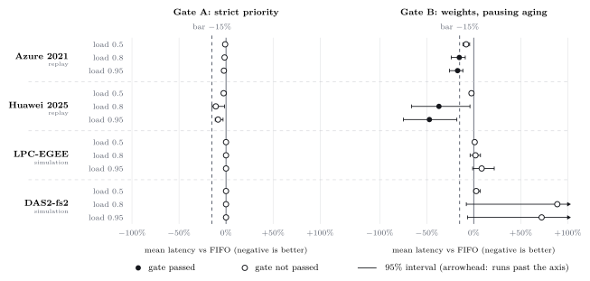
**Figure 12.** Trace results: mean latency against FIFO at offered loads 0.5, 0.8 and 0.95, for predictive routing as built (gate A) and with worker-time weights and pausing aging (gate B). Azure and Huawei were replayed through the real broker (28 windows, block bootstrap; Huawei pooled over three repeats); LPC-EGEE and DAS2-fs2 were simulated (seven windows). Each dot is a cell’s point estimate and each line its 95% interval, clipped at $\pm$ 100% with an arrowhead where it runs past (DAS2-fs2 at loads 0.8 and 0.95 reaches $+$ 213% and $+$ 156%). The dashed line is the pre-registered $-$ 15% bar; a filled dot passed its gate and a hollow one did not, and a gate also needs its guardrails, so a dot left of the bar can still be hollow. The numbers, with margins, are in Table 16.

What makes the serverless traces work is that their keys recur and are predictable. On Azure a per-key median predicts a held-out duration to within a typical factor of 1.3, against 29 for a single global median (Table 8); the keys that carry most jobs are the same functions over and over. The two HPC logs are the opposite case, and the results there are the clearest failures in the paper. They are simulations, since we did not replay them (6), but the simulator matched the broker on the two traces we did replay (Section 5.6). On LPC-EGEE only 21% of the 117,823 evaluated jobs got a prediction at load 0.8: 24% belonged to keys that were too new and 53% to keys whose history had expired. Of those stale-key jobs, 89% had themselves waited more than a minute, which suggests that many keys were not idle so much as stuck behind a backlog that delivered no fresh completions. Most jobs therefore took the default level, and the weighted design stayed close to FIFO, with mean latency 1.0% to 8.5% above FIFO’s and intervals that included zero. On DAS2-fs2 most jobs did get a prediction, but the predictions were about as good as a global median, and acting on them hurt. At load 0.8 the design with weights and pausing aging raised mean latency by 88.8% on average across the seven windows, an interval of [ $-$ 7.9, $+$ 213.1]% that includes zero (pooled over all jobs the rise was 44%): short jobs gained several-fold, but long jobs carry most of the work, and they waited several times longer, so that the guardrails failed with the all-message P99 at 2.61 $\times$ FIFO’s and an upper bound of 5.1 $\times$ . The oracle with the same scheduler improved every window there, with a mean reduction of 30.1%. The scheduler is therefore not the problem. An exploratory diagnosis, run afterwards and not pre-registered, points at the predictor and at the aging time scale. With the predictor’s levels and no aging, short jobs gained but medium jobs slowed by 44% and long jobs waited about twice as long, whereas with the oracle’s levels medium jobs became faster. And a pausing rule with a five-second threshold moves thousands of jobs, large mispredicted ones included, upward during waits of hours: with weights and no aging the predictor was 7% better than FIFO, and with pausing aging 44% worse. Scaling the aging threshold to the workload was not tested.

**Table 8.** Predicting held-out Azure Functions durations: median absolute $\log_2$ error, share within a factor of 2, and tier accuracy.
Predictor	Median $\|\log_2\|$ error	Within 2 $\times$	Tier acc.
Global median	4.84	10%	57%
Per-key median	0.39	62%	79%
Per-key median, with gates	0.43	59%	74%

Two further results are negative. We tested whether size-binned keys, which split a job type by the size of its input, would improve prediction under load. They did improve the predictor’s accuracy, but mean latency changed by only $+$ 0.7% [ $+$ 0.5, $+$ 0.9] against job-type keys, which missed the pre-registered bar, and for one job type whose cost does not follow its size it got 8.7% worse. The AWS replication agreed: mean latency changed by $-$ 1.5% [ $-$ 4.5, $+$ 0.4], again short of the bar, and the invoice job was 9.5% worse. And before settling on statistics we compared eight online learners, including River models, against per-key statistics and simple baselines offline. None of them passed both quality criteria on every workload, with the strict rule that a model be no worse than both baselines everywhere and no tolerance for noise. As Section 6 says, the workload gave a model little to find, so this is evidence that statistics suffice here, not that learning cannot help.

5.3 Switching aging off

If aging is what limits the gain, switching it off should recover it. Two experiments test that. On the production flow on AWS, with ten seeds, predictive routing with aging off cut mean latency by 37.4% against predictive routing with the default aging (interval $-$ 37.4% [ $-$ 39.8, $-$ 35.1]), which puts it 57.6% below FIFO, about the size of the RabbitMQ sidecar’s gain (a different baseline and host layout, so not a tested comparison). The cost was a rise against FIFO of 13.6% in all-message P99 and 13.6% in the longest wait of a long job, in runs of five minutes that cannot show starvation. And on Huawei Cloud through the real broker (9), predictive routing with aging off passed gate A’s rules at both loads, with mean latency 37.4% and 45.4% below FIFO’s, where the default aging failed with 11.0% and 8.5%. At load 0.8 the whole-run mean fell from 17.7 s under FIFO and 14.8 s under the default aging to 1.7 s. The all-message P99 stayed within 1.12 $\times$ of FIFO’s and the longest wait of a long job within 1.16 $\times$ , and the three repeats agreed. A Huawei cell lasts about twenty-five minutes, so this cannot show starvation over hours either, and aging is the protection against it. The weighted design, which keeps a pausing form of aging, is the safer version of the same fix. This experiment ran on two smaller hosts than the main replay and carries its own FIFO and predictive arms, so its numbers are not tested against the main replay’s.

**Table 9.** Aging switched off, Huawei Cloud replayed through the real broker (three repeats, 28 windows, block bootstrap). Default aging is gate A; the same predictor with aging off is gate N, with the same three rules.
	Default aging (gate A)		Aging off (gate N)			Gate N guardrails
2-3(lr)4-5(lr)7-8 Load	Mean vs FIFO	Passed	Mean vs FIFO	Passed	Off vs default	P99	Long wait
0.8	$-$ 11.0% [ $-$ 15.1, $-$ 1.7]	no	$-$ 37.4% [ $-$ 66.0, $-$ 4.4]	yes	$-$ 34.1%	1.07 $\times$	1.16 $\times$
0.95	$-$ 8.5% [ $-$ 11.7, $-$ 3.2]	no	$-$ 45.4% [ $-$ 73.6, $-$ 16.2]	yes	$-$ 41.8%	1.12 $\times$	1.14 $\times$

5.4 Baselines and ablation

A reader’s first question is whether the predictor is needed at all. We tested simple alternatives on the production flow on AWS, with ten seeds and readings fixed before the run (Table 10). Predictive routing again reduced mean latency by 32.1% against FIFO and beat the hand-tuned map by 15.5%. But a queue per job type, served in equal shares of worker time with no prediction at all, had a mean latency 42.1% below predictive routing’s. Its all-message P99 was 51.7% higher, because its slowest classes wait longer, and it needs an operator to create one queue per type, which does not scale to the hundreds of keys of a serverless trace. This workload is that design’s best case, nine job types of nearly fixed cost, so the predictor’s advantage here is that it needs no per-type queues, not that it schedules better. Summarising a key by its mean or its 75th percentile instead of its median made predictive routing 3.6% and 3.8% worse. Removing any one of the four predictor components changed mean latency over the whole run by less than three percent, and the intervals after the cost shift were too wide to decide (Table 11). This workload’s costs are stable and its keys active, so it cannot show what those components were built for, and we do not claim they help on it.

**Table 10.** Baselines and aging isolation on the production flow, on AWS, ten seeds. Medians over seeds for the levels; the two change columns are the means of the per-seed paired changes in mean latency, each relative to the column’s base, so the hand-tuned map’s change against predictive routing is not the negative of predictive routing’s change against the map. Descriptive; the pre-registered readings are in the text.
Arm	Mean (s)	vs FIFO	vs predictive	Short P50 (ms)	P99 (s)	Long wait (s)
FIFO	6.93	—	$+$ 47.7%	4965	21.1	20.8
Predictive routing	4.78	$-$ 32.1%	—	39	21.8	21.7
Hand-tuned static map	5.61	$-$ 19.6%	$+$ 18.5%	450	21.5	26.1
Queue per job type, no prediction	2.73	$-$ 60.8%	$-$ 42.1%	16	32.0	2.9
Predictive, aging off	2.92	$-$ 57.6%	$-$ 37.4%	15	24.0	23.9
Predictive, mean summary	4.90	$-$ 29.7%	$+$ 3.6%	42	21.6	21.6
Predictive, 75th-percentile summary	4.90	$-$ 29.6%	$+$ 3.8%	41	21.7	21.6

**Table 11.** Removing one predictor component on the production flow (change in mean latency against the full predictor, ten seeds, 95% bootstrap interval). “No effect shown” means the whole interval lies within $\pm 3\%$ ; “inconclusive” means it does not.
	Whole run		After the cost shift
2-3(lr)4-5 Component removed	Change	Reading	Change	Reading
Decay and idle forgetting	$0.0$ % [ $-$ 2.1, $+$ 2.3]	no effect shown	$+$ 1.0% [ $-$ 3.6, $+$ 6.1]	inconclusive
99th-percentile spread check	$+$ 0.1% [ $-$ 0.4, $+$ 0.6]	no effect shown	$+$ 1.0% [ $-$ 1.5, $+$ 3.9]	inconclusive
Staleness rule	$+$ 0.4% [ $-$ 0.2, $+$ 1.1]	no effect shown	$+$ 2.1% [ $-$ 0.8, $+$ 6.1]	inconclusive
Minimum of 20 observations	$+$ 0.2% [ $-$ 1.1, $+$ 2.0]	no effect shown	$+$ 1.7% [ $-$ 0.7, $+$ 4.1]	inconclusive

5.5 Parameter sensitivity

The predictor’s and aging’s parameters were fixed by judgement. We varied each in turn, in the simulator at load 0.8 on both traces (12; 18 variants including the defaults, with the values listed in the pre-registration). The weighted design’s gate was robust: it passed in 18 of 18 variants on Huawei and 16 on Azure, failing on Azure only with 100 minimum observations and with two levels. Predictive routing as built was fragile. On Azure it passed in 0 variants, and on Huawei its default sits at the bar ( $-$ 15.0% against a limit of $-$ 15%) and its verdict flips under 8 of the other variants. The aging threshold dominates: Huawei’s gate-A change is $-$ 3.3% with a one-second threshold, $-$ 15.0% at the default five seconds and $-$ 40.7% at thirty. These are simulator results. The simulator matched the broker on both traces (Section 5.6), but we did not rerun the variants through the broker, apart from the extreme of switching aging off above.

**Table 12.** One-at-a-time parameter sensitivity in the simulator at load 0.8 (seven windows): whether each parameter moves the gate’s mean-latency verdict away from its verdict at the defaults, and at which value. Simulator results only; the grid is in the text. Azure’s gate A fails at every value, so “robust” there means it never passes.
	Azure 2021		Huawei Cloud
2-3(lr)4-5 Parameter	Gate A	Gate B	Gate A	Gate B
Minimum observations	robust	flips at 100	flips at 5, 100	robust
Spread ratio	robust	robust	flips at 4	robust
Decay	robust	robust	flips at 0.98, 0.999, 1.0	robust
Staleness limit	robust	robust	robust	robust
Aging threshold	robust	robust	flips at 1s	robust
Level weights	robust	robust	robust	robust
Number of levels	robust	flips at 2	flips at 2	robust
Variants passing (of 18)	0	16	10	18

5.6 The simulator against the real broker

The replay lets us check the simulator on the traces (13). Whole-run mean-latency changes agree to within 1.3 points in every arm and cell, with a median gap of 0.5 points, including the weighted oracle, which both put more than sixty percent below FIFO on Huawei at loads 0.8 and 0.95. That is the opposite of the production flow, where the simulator overstated predictive routing’s gain by about 41%. The difference is the handlers: the production flow’s do real CPU work on four workers, which the simulator does not model, and the replay’s only sleep. So the agreement shows that the simulator’s queueing is right, and it does not show that a real application with CPU-bound handlers would match it. The broker’s own cost is small at light load: a job on Huawei took a median of 0.5 ms (P99 1.3 ms) longer than its duration, and on Azure 4.1 ms (6.8 ms), in trace time.

**Table 13.** Mean-latency change against FIFO over each whole run (the mean over all jobs of the evaluation half, not the window average of 16), measured through the real broker and predicted by the simulator, for the same arms, traces and loads. Azure’s strict-priority arm is omitted because it changes nothing in either (a few hundredths of a point), and the weighted oracle ran at load 0.8 on Azure only.
		Predictive		Weighted		Weighted oracle
3-4(lr)5-6(lr)7-8 Trace	Load	Replay	Simulator	Replay	Simulator	Replay	Simulator
Azure	0.5	—	—	$-$ 10.3%	$-$ 11.3%	—	—
Azure	0.8	—	—	$-$ 7.9%	$-$ 7.7%	$-$ 52.8%	$-$ 52.8%
Azure	0.95	—	—	$-$ 9.3%	$-$ 8.8%	—	—
Huawei	0.5	$-$ 11.4%	$-$ 10.6%	$-$ 10.9%	$-$ 9.6%	$-$ 7.8%	$-$ 7.0%
Huawei	0.8	$-$ 16.3%	$-$ 16.9%	$-$ 90.4%	$-$ 89.7%	$-$ 61.8%	$-$ 61.7%
Huawei	0.95	$-$ 9.5%	$-$ 9.8%	$-$ 83.2%	$-$ 82.8%	$-$ 66.7%	$-$ 66.6%

5.7 Conditions of the local runs

The local production-flow figures in this paper, and those for the aging guardrails and the size bins, come from a quiet-machine re-run: the three wall-clock matrices were repeated on a laptop with turbo disabled and the clock capped at 2.3 GHz, with the same frozen configurations and analysis, and the simulations were re-run too. We use the re-run because its conditions are documented and it was much less noisy. No pre-registered verdict differs from the original runs, and all four simulations reproduced byte for byte. Effect sizes do depend on CPU speed, because job sizes and arrival rates are fixed and a slower CPU is a heavier load. The original local run’s kernels were 1.6 to 1.8 times faster than the re-run’s, and there the mean fell by 27.9% against FIFO, the short-job median by 88.4% and producer-only keys by 15.4%, against 25.6%, 57.7% and 10.5% here; the longer backlog gives the default aging more to promote, which hurts the short-job median most. Load relative to CPU speed therefore matters as much as the policy, and the AWS replication, whose CPU was about twice as fast as the re-run’s, is the independent check.

6 Limitations and threats to validity

The most important limitation is the kind of evidence. Everything in this paper is synthetic or trace-driven, and we have no production workload. The production-flow scenario was written by us, and the traces, though real, are simulated or, for Azure and Huawei, replayed through the real broker with handlers that sleep for the recorded duration and so do no work, which removes the contention that real handlers cause: arrivals are reconstructed where a trace does not record them, and the Huawei timestamps are completion times, so the arrival process we replay is an inference. For Azure, arrival is the end timestamp minus the duration, from timestamps the dataset authors modified, and the 2% of rows that share an arrival time are ordered as the converted file lists them, which alone moves the weighted arms by up to 2.5%. The simulator also makes modelling choices that real platforms do not: it queues on 64 workers and scales arrivals to a target load, where a serverless platform would scale out instead. A parallel job on DAS2-fs2 occupies one simulated worker, LPC-EGEE is restricted to single-processor jobs, and the Huawei trace is one region on one day. The experiments ran in one cloud provider, one region and two instance types, which gives a low-latency network and says nothing about a wide-area deployment. The thirty-minute run has only two repetitions, so its checks are per repetition and carry no intervals. The Azure replay ran once per cell, so it carries no measure of run-to-run noise (Huawei’s three repeats agreed to within a few percent, and no cell was unstable), and its load-0.8 gate passes by 0.3 points. Two of the 76 replay cells lost the broker within seconds of starting, one on each pair of hosts, and were re-run once as pre-registered; both retries are valid, but we do not know the cause, and it may be a rare startup defect in the broker. The aging-off replay ran on smaller hosts than the main replay. We did not replay the two research-cluster logs, whose results are simulated. The local production-flow results depend on CPU speed, as the comparison with the original run in Section 5 shows, so that run’s absolute effect sizes should not be carried to other hardware.

We checked the simulator against the broker twice. The first check is on the production flow, the only workload of ours whose handlers do real computation. The measured production-flow runs, local and AWS, were replayed through the simulator with their own arrivals and handler durations, under criteria frozen before the run (Table 5; the pre-registration is v4-simvalidation-1). The simulator reproduced the direction of predictive routing’s effect in every phase and the order of the policies in all 5 seeds of both sets, but it failed the bar for the size of the effect: against FIFO it reported a mean-latency reduction of 37.0% for predictive routing where the broker achieved 25.6% locally, and 42.7% against 30.8% on AWS, and its gap was 11.4 to 13.1 points for predictive routing and the oracle against a limit of 10. In relative terms it overstated the reduction by about 41%. Its absolute latencies were only 0.31 to 0.41 of the measured ones. We did not tune the simulator in response. The simulator has no broker overhead, and it replays each message once, so the work of the retried messages of the failing job type is missing. The second check came later, on the traces themselves: the Azure and Huawei traces were replayed through the broker, and the simulator agreed with it to within 1.3 points in every arm and cell (Section 5.6). The checks differ in what the workload does. The production flow’s handlers compute, and the replayed handlers sleep, so the replay tests the simulator’s queueing and cannot test the effect of contention. We therefore read the replayed traces’ results as measured and the two research-cluster logs’ as simulated, with their directions and the ordering of policies supported, and their sizes uncertain by as much as the production-flow check suggests for work that computes.

Some limitations come from how the design learns. Durations are learned from handlers that succeeded, so a key whose slow cases fail looks faster than it is. The predictor’s parameters (1) were fixed by judgement and varied only afterwards, one at a time and in the simulator (5.5); we did not rerun the variants through the broker, so how sensitive the real-broker results are is not measured, and the weighted design was built in response to the Azure result, so that trace is in-sample for it (Table 5). The budgets of the first experiment were set after seeing earlier offline data, as Section 4 says, so that gate is less independent than the later ones. And the evidence about learned models is narrow: the offline comparison used a workload whose only feature was a three-valued category, which leaves a per-key average close to the best possible predictor and little for a richer model to find. We conclude that statistics were enough for these workloads, not that models never help.

Others come from the scheduler. A non-preemptive queue cannot shorten a long job’s own service time, so we make no claim that all-message tail latency improves; in the production flow it stays within 1.03 $\times$ of FIFO’s. The tails of individual classes do move, by about 45% down for the cheapest classes and by about 5% up for the mid-cost ones (9). Where long jobs carry most of the work, favouring short ones can make the overall result worse, as the DAS2 log shows. The comparison with a queue per job type is on one workload, which is that design’s best case, nine job types of nearly fixed cost; we did not test it where types are many or costs vary within a type. The broker is a prototype with in-memory state and no durability, authentication or backpressure, and it had the lowest throughput of the three brokers we measured. The comparison with RabbitMQ is also bounded by our configuration: RabbitMQ 3.12 ran with classic priority queues and a prefetch of one, which is how priorities take effect at all, and which limits its throughput. Kafka, Pulsar, managed queues and durable modes were out of scope, and we did not run Alibaba’s GPU traces.

Finally, the code, configurations, pre-registrations and result files are in the repository at https://github.com/divyanshusingh2903/predictive-multi-level-message-queue, with the raw per-message data archived outside git and hashed with SHA-256, so that the published files can be checked against them. The version described here is the release tagged v0.2.0-preprint.

Use of AI assistance.

AI models were involved in the code, in running the tests and benchmarks, and in writing this paper. The models were Claude Sonnet 5.5, Claude Opus 5.5, ChatGPT Sol 6, Sol 6.1 and Luna 6, used through Claude Code and through Forge, a custom open-source fork of Opencode. The author directed the work, reviewed the results and the text, and is responsible for the content.

7 Conclusion

Learning each message key’s duration from the acknowledgements a broker already receives is enough to schedule shortest-expected-first without any per-endpoint configuration. On a production-style workload it beats FIFO and hand-tuned priorities, and it does so on separate cloud hardware and against RabbitMQ and Redis. But the predictor is not the most important part. Under sustained backlogs the broker’s default aging appears to erase the order that the predictor produces: predictive routing as built failed in every cell of the Azure and Huawei replays, passed on Huawei once aging was switched off (a test we ran on Huawei and the production flow only), and, with an aging design built for overload, passed in four of six cells. Where job types are few and stable, a queue per type does better on the mean with no prediction at all, and on one stable trace a static map from history did as well; the predictor’s case is that it needs neither. It needs keys that recur and predict well, which serverless functions have and the two HPC logs largely lack, and where keys do not predict well, or where long jobs carry most of the work, it does not help and can hurt. We make no claim about tail latency, and learned models remain untested against workloads rich enough to need them.

A Pre-registered criteria

The pass/fail record and pre-registered bars behind 8, Figure 10, 12 (Table 14, 15, Table 16), and the closed-form values plotted in Figure 11 (18).

**Table 14.** Production-flow benchmark: local quiet-machine re-run and its replication on AWS. Point estimates with 95% bootstrap intervals, paired over five seeds. Margin is the distance inside the bar (negative: outside), taken at the quantity the rule tests: the point estimate for the improvement bars (P1, P2, S4), the interval’s upper end for the guardrails and S1, and the upper end against zero for S2.
Criterion	Bar	Local run			AWS replication
3-5(lr)6-8		Estimate [95% CI]	Margin	Result	Estimate [95% CI]	Margin	Result
P1 mean vs FIFO	$\le -15\%$	$-$ 25.6% [ $-$ 29.4, $-$ 21.8]	$+$ 10.6 pts	pass	$-$ 30.8% [ $-$ 35.3, $-$ 27.1]	$+$ 15.8 pts	pass
P2 short-class P50 vs FIFO	$\le -30\%$	$-$ 57.7% [ $-$ 70.0, $-$ 45.3]	$+$ 27.7 pts	pass	$-$ 94.8% [ $-$ 99.0, $-$ 86.5]	$+$ 64.8 pts	pass
G1 all-message P99 vs FIFO	$\le 1.25\times$	1.02 $\times$ [1.00, 1.05]	$+$ 0.20 $\times$	pass	1.03 $\times$ [1.02, 1.05]	$+$ 0.20 $\times$	pass
G2 long max wait vs FIFO	$\le 2\times$	0.99 $\times$ [0.95, 1.03]	$+$ 0.97 $\times$	pass	0.99 $\times$ [0.90, 1.05]	$+$ 0.95 $\times$	pass
S1 vs hand-tuned static	$\le +10\%$	$-$ 11.1% [ $-$ 13.4, $-$ 8.7]	$+$ 18.7 pts	pass	$-$ 14.4% [ $-$ 18.4, $-$ 10.7]	$+$ 20.7 pts	pass
S2 vs misconfigured static	interval $<0$	$-$ 30.1% [ $-$ 34.3, $-$ 26.0]	$+$ 26.0 pts	pass	$-$ 36.8% [ $-$ 41.1, $-$ 33.2]	$+$ 33.2 pts	pass
S4 producer keys vs FIFO	$\le -5\%$	$-$ 10.5% [ $-$ 12.0, $-$ 8.8]	$+$ 5.5 pts	pass	$-$ 15.7% [ $-$ 17.1, $-$ 14.6]	$+$ 10.7 pts	pass

**Table 15.** Harbinger against RabbitMQ and Redis on the same workload, on AWS. Margin is the distance inside the bar (negative: outside), as in 14; for the equivalence bar S1 it is the distance of the interval’s farther end from the limit.
Criterion	Bar	Estimate [95% CI]	Margin	Result
P1 mean vs RabbitMQ FIFO	$\le -15\%$	$-$ 21.7% [ $-$ 26.2, $-$ 18.4]	$+$ 6.7 pts	pass
P3 mean vs Redis FIFO	$\le -15\%$	$-$ 25.5% [ $-$ 29.5, $-$ 22.6]	$+$ 10.5 pts	pass
P2 short-class P50 vs RabbitMQ FIFO	$\le -30\%$	$-$ 89.5% [ $-$ 98.8, $-$ 75.5]	$+$ 59.5 pts	pass
G1 all-message P99 vs RabbitMQ FIFO	$\le 1.25\times$	1.10 $\times$ [1.07, 1.12]	$+$ 0.13 $\times$	pass
S1 Harbinger FIFO vs RabbitMQ FIFO	$\pm 10\%$	$+$ 11.0% [ $+$ 10.4, $+$ 11.6]	$-$ 1.6 pts	fail
S3 sidecar on RabbitMQ vs RabbitMQ FIFO	$\le -15\%$	$-$ 57.6% [ $-$ 58.6, $-$ 56.8]	$+$ 42.6 pts	pass
S6 weighted aging vs RabbitMQ FIFO	$\le -15\%$	$-$ 52.4% [ $-$ 53.4, $-$ 51.0]	$+$ 37.4 pts	pass
S8 RabbitMQ priority, long-class max wait	$\le 2\times$	5.23 $\times$ [4.79, 5.55]	$-$ 3.55 $\times$	fail

**Table 16.** Trace results, mean latency against FIFO and whether each pre-registered gate passed. Azure and Huawei were replayed through the real broker on AWS (28 windows, block bootstrap, Huawei pooled over three repeats); the two research-cluster logs were simulated (seven windows). A: predictive routing as built. B: with worker-time weights and pausing aging. Mean vs FIFO is the average of the per-window paired changes, as gated; the whole-run changes of Table 13 differ (Section 4). Margin is how many points the point estimate lies beyond the $-15\%$ bar (negative: short of it); a pass also needs the interval to exclude zero and the guardrails to hold, so a positive margin is not by itself a pass, and the upper end of the interval is the cut the data support with confidence.
		Gate A: strict priority			Gate B: weights, pausing aging
3-5(lr)6-8 Trace	Load	Change [95% CI]	Margin	Passed	Change [95% CI]	Margin	Passed
Azure 2021, replay	0.5	$-$ 0.9% [ $-$ 1.9, $-$ 0.2]	$-$ 14.1 pts	no	$-$ 8.0% [ $-$ 11.5, $-$ 4.3]	$-$ 7.0 pts	no
Azure 2021, replay	0.8	$-$ 1.6% [ $-$ 3.0, $-$ 0.6]	$-$ 13.4 pts	no	$-$ 15.3% [ $-$ 23.9, $-$ 9.0]	$+$ 0.3 pts	yes
Azure 2021, replay	0.95	$-$ 2.2% [ $-$ 3.9, $-$ 1.1]	$-$ 12.8 pts	no	$-$ 17.2% [ $-$ 25.8, $-$ 11.6]	$+$ 2.2 pts	yes
Huawei 2025, replay	0.5	$-$ 2.5% [ $-$ 4.6, 0.0]	$-$ 12.5 pts	no	$-$ 2.4% [ $-$ 4.4, 0.0]	$-$ 12.6 pts	no
Huawei 2025, replay	0.8	$-$ 10.9% [ $-$ 14.8, $-$ 1.6]	$-$ 4.1 pts	no	$-$ 37.0% [ $-$ 66.0, $-$ 4.0]	$+$ 22.0 pts	yes
Huawei 2025, replay	0.95	$-$ 8.4% [ $-$ 11.5, $-$ 3.2]	$-$ 6.6 pts	no	$-$ 47.1% [ $-$ 74.8, $-$ 17.9]	$+$ 32.1 pts	yes
LPC-EGEE, simulation	0.5	$0.0$ % (none)	$-$ 15.0 pts	no	$+$ 1.0% [ $-$ 0.7, $+$ 2.8]	$-$ 16.0 pts	no
LPC-EGEE, simulation	0.8	$0.0$ % (none)	$-$ 15.0 pts	no	$+$ 1.9% [ $-$ 3.8, $+$ 7.2]	$-$ 16.9 pts	no
LPC-EGEE, simulation	0.95	$0.0$ % (none)	$-$ 15.0 pts	no	$+$ 8.5% [ $-$ 1.1, $+$ 21.8]	$-$ 23.5 pts	no
DAS2-fs2, simulation	0.5	$0.0$ % (none)	$-$ 15.0 pts	no	$+$ 2.7% [0.0, $+$ 6.8]	$-$ 17.7 pts	no
DAS2-fs2, simulation	0.8	$0.0$ % (none)	$-$ 15.0 pts	no	$+$ 88.8% [ $-$ 7.9, $+$ 213.1]	$-$ 103.8 pts	no
DAS2-fs2, simulation	0.95	$0.0$ % (none)	$-$ 15.0 pts	no	$+$ 72.2% [ $-$ 6.6, $+$ 155.6]	$-$ 87.2 pts	no

**Table 17.** The same two traces in the simulator, as first run (seven independent windows), before the replay. Gate A passed in one of six cells and gate B in five. Margin as in Table 16.
		Gate A: strict priority			Gate B: weights, pausing aging
3-5(lr)6-8 Trace	Load	Change [95% CI]	Margin	Passed	Change [95% CI]	Margin	Passed
Azure 2021	0.5	$-$ 0.7% [ $-$ 1.5, $-$ 0.1]	$-$ 14.3 pts	no	$-$ 15.4% [ $-$ 25.8, $-$ 5.4]	$+$ 0.4 pts	yes
Azure 2021	0.8	$-$ 0.9% [ $-$ 2.0, $-$ 0.1]	$-$ 14.1 pts	no	$-$ 22.8% [ $-$ 37.2, $-$ 9.3]	$+$ 7.8 pts	yes
Azure 2021	0.95	$-$ 1.2% [ $-$ 2.8, $-$ 0.2]	$-$ 13.8 pts	no	$-$ 25.3% [ $-$ 40.3, $-$ 10.6]	$+$ 10.3 pts	yes
Huawei 2025	0.5	$-$ 4.8% [ $-$ 13.8, $-$ 0.1]	$-$ 10.2 pts	no	$-$ 4.3% [ $-$ 12.5, 0.0]	$-$ 10.7 pts	no
Huawei 2025	0.8	$-$ 15.0% [ $-$ 27.0, $-$ 4.2]	$+$ 0.0 pts	yes	$-$ 46.5% [ $-$ 78.3, $-$ 13.3]	$+$ 31.5 pts	yes
Huawei 2025	0.95	$-$ 7.9% [ $-$ 11.2, $-$ 4.5]	$-$ 7.1 pts	no	$-$ 49.9% [ $-$ 77.4, $-$ 21.1]	$+$ 34.9 pts	yes

**Table 18.** Mean waiting time under non-preemptive priority, relative to FIFO, from the closed forms of Section Section 5.1. An illustration of the model, not a measurement. Short-job share $p$ , long-to-short size ratio $r$ , load $\rho$ , and the short class’s share of the work $\pi$ .
				Mean wait relative to FIFO
5-7 $p$	$r$	$\rho$	$\pi$	Short class	Long class	All jobs
0.9	10	0.5	47%	0.66	1.31	0.72
0.9	10	0.8	47%	0.32	1.61	0.45
0.9	10	0.95	47%	0.09	1.82	0.26
0.9	100	0.5	8%	0.52	1.04	0.57
0.9	100	0.8	8%	0.21	1.07	0.30
0.9	100	0.95	8%	0.05	1.09	0.16
0.5	100	0.5	1%	0.50	1.00	0.75
0.5	100	0.8	1%	0.20	1.01	0.60
0.5	100	0.95	1%	0.05	1.01	0.53

References

Amazon Web Services. 2026a. Amazon SQS Queue Types. Amazon SQS Developer Guide. https://docs.aws.amazon.com/AWSSimpleQueueService/latest/SQSDeveloperGuide/sqs-queue-types.html.

Amazon Web Services. 2026b. Creating and Configuring an Amazon SQS Event Source Mapping. AWS Lambda Developer Guide. https://docs.aws.amazon.com/lambda/latest/dg/services-sqs-configure.html.

Bansal, Nikhil, and Mor Harchol-Balter. 2001. “Analysis of SRPT Scheduling: Investigating Unfairness.” ACM SIGMETRICS. https://doi.org/10.1145/378420.378792.

Celery Project. 2026. Routing Tasks: Redis Message Priorities. Celery documentation. https://docs.celeryq.dev/en/main/userguide/routing.html.

Cobham, Alan. 1954. “Priority Assignment in Waiting Line Problems.” Journal of the Operations Research Society of America 2 (1): 70–76. https://doi.org/10.1287/opre.2.1.70.

Dean, Jeffrey, and Luiz André Barroso. 2013. “The Tail at Scale.” Communications of the ACM 56 (2): 74–80. https://doi.org/10.1145/2408776.2408794.

Dell’Amico, Matteo, Damiano Carra, Mario Pastorelli, and Pietro Michiardi. 2014. “Revisiting Size-Based Scheduling with Estimated Job Sizes.” IEEE International Symposium on Modeling, Analysis and Simulation of Computer and Telecommunication Systems (MASCOTS). https://doi.org/10.1109/MASCOTS.2014.57.

Didona, Diego, and Willy Zwaenepoel. 2019. “Size-Aware Sharding for Improving Tail Latencies in in-Memory Key-Value Stores.” USENIX Symposium on Networked Systems Design and Implementation (NSDI). https://www.usenix.org/conference/nsdi19/presentation/didona.

Feitelson, Dror G., Dan Tsafrir, and David Krakov. 2014. “Experience with Using the Parallel Workloads Archive.” Journal of Parallel and Distributed Computing 74 (10): 2967–82. https://doi.org/10.1016/j.jpdc.2014.06.013.

Fu, Yichao, Siqi Zhu, Runlong Su, Aurick Qiao, Ion Stoica, and Hao Zhang. 2024. “Efficient LLM Scheduling by Learning to Rank.” Advances in Neural Information Processing Systems (NeurIPS). https://arxiv.org/abs/2408.15792.

Fu, Yuqi, Li Liu, Haoliang Wang, Yue Cheng, and Songqing Chen. 2022. “SFS: Smart OS Scheduling for Serverless Functions.” International Conference for High Performance Computing, Networking, Storage and Analysis (SC). https://doi.org/10.1109/SC41404.2022.00047.

Fu, Yuqi, Ruizhe Shi, Haoliang Wang, Songqing Chen, and Yue Cheng. 2024. “ALPS: An Adaptive Learning, Priority OS Scheduler for Serverless Functions.” USENIX Annual Technical Conference (ATC). https://www.usenix.org/conference/atc24/presentation/fu.

Gan, Yu, Yanqi Zhang, Dailun Cheng, et al. 2019. “An Open-Source Benchmark Suite for Microservices and Their Hardware-Software Implications for Cloud & Edge Systems.” ACM International Conference on Architectural Support for Programming Languages and Operating Systems (ASPLOS). https://doi.org/10.1145/3297858.3304013.

Gaussier, Eric, David Glesser, Valentin Reis, and Denis Trystram. 2015. “Improving Backfilling by Using Machine Learning to Predict Running Times.” International Conference for High Performance Computing, Networking, Storage and Analysis (SC). https://doi.org/10.1145/2807591.2807646.

Gittins, John C. 1979. “Bandit Processes and Dynamic Allocation Indices.” Journal of the Royal Statistical Society, Series B 41: 148–64. https://doi.org/10.1111/j.2517-6161.1979.tb01068.x.

Gu, Juncheng, Mosharaf Chowdhury, Kang G. Shin, et al. 2019. “Tiresias: A GPU Cluster Manager for Distributed Deep Learning.” USENIX Symposium on Networked Systems Design and Implementation (NSDI). https://www.usenix.org/conference/nsdi19/presentation/gu.

Harchol-Balter, Mor, Mark E. Crovella, and Cristina D. Murta. 1999. “On Choosing a Task Assignment Policy for a Distributed Server System.” Journal of Parallel and Distributed Computing 59 (2): 204–28. https://doi.org/10.1006/jpdc.1999.1577.

Harchol-Balter, Mor, Bianca Schroeder, Nikhil Bansal, and Mukesh Agrawal. 2003. “Size-Based Scheduling to Improve Web Performance.” ACM Transactions on Computer Systems 21 (2): 207–33. https://doi.org/10.1145/762483.762486.

Joosen, Artjom, Ahmed Hassan, Martin Asenov, et al. 2023. “How Does It Function? Characterizing Long-Term Trends in Production Serverless Workloads.” Proceedings of the 2023 ACM Symposium on Cloud Computing (SoCC), 443–58. https://doi.org/10.1145/3620678.3624783.

Joosen, Artjom, Ahmed Hassan, Martin Asenov, et al. 2025. “Serverless Cold Starts and Where to Find Them.” Proceedings of the Twentieth European Conference on Computer Systems (EuroSys), 938–53. https://doi.org/10.1145/3689031.3696073.

Kaffes, Kostis, Timothy Chong, Jack Tigar Humphries, Adam Belay, David Mazières, and Christos Kozyrakis. 2019. “Shinjuku: Preemptive Scheduling for

\mu

Second-Scale Tail Latency.” USENIX Symposium on Networked Systems Design and Implementation (NSDI). https://www.usenix.org/conference/nsdi19/presentation/kaffes.

Kaffes, Kostis, Neeraja J. Yadwadkar, and Christos Kozyrakis. 2022. “Hermod: Principled and Practical Scheduling for Serverless Functions.” ACM Symposium on Cloud Computing (SoCC). https://doi.org/10.1145/3542929.3563468.

Kleinrock, Leonard. 1965. “A Conservation Law for a Wide Class of Queueing Disciplines.” Naval Research Logistics Quarterly 12 (2): 181–92. https://doi.org/10.1002/nav.3800120206.

Kreps, Jay, Neha Narkhede, and Jun Rao. 2011. “Kafka: A Distributed Messaging System for Log Processing.” NetDB Workshop.

Lu, Dong, Huanyuan Sheng, and Peter Dinda. 2004. “Size-Based Scheduling Policies with Inaccurate Scheduling Information.” IEEE International Symposium on Modeling, Analysis and Simulation of Computer and Telecommunication Systems (MASCOTS). https://doi.org/10.1109/MASCOT.2004.1348179.

Mao, Hongzi, Malte Schwarzkopf, Shaileshh Bojja Venkatakrishnan, Zili Meng, and Mohammad Alizadeh. 2019. “Learning Scheduling Algorithms for Data Processing Clusters.” ACM SIGCOMM. https://doi.org/10.1145/3341302.3342080.

Microsoft. 2026a. Priority Queue Pattern. Azure Architecture Center. https://learn.microsoft.com/azure/architecture/patterns/priority-queue.

Microsoft. 2026b. Queue-Based Load Leveling Pattern. Azure Architecture Center. https://learn.microsoft.com/azure/architecture/patterns/queue-based-load-leveling.

Mitzenmacher, Michael. 2020. “Scheduling with Predictions and the Price of Misprediction.” Innovations in Theoretical Computer Science (ITCS). https://doi.org/10.4230/LIPIcs.ITCS.2020.14.

Mitzenmacher, Michael, and Rana Shahout. 2025. “Queueing, Predictions, and Large Language Models: Challenges and Open Problems.” Stochastic Systems 15 (3): 195–219. https://doi.org/10.1287/stsy.2025.0106.

Mitzenmacher, Michael, and Sergei Vassilvitskii. 2022. “Algorithms with Predictions.” Communications of the ACM 65 (7): 33–35. https://doi.org/10.1145/3528087.

Montiel, Jacob, Max Halford, Saulo Martiello Mastelini, et al. 2021. “River: Machine Learning for Streaming Data in Python.” Journal of Machine Learning Research 22 (110): 1–8. https://jmlr.org/papers/v22/20-1380.html.

Nanavati, Akshay, and Girish Joshi. 2021. FOQS: Scaling a Distributed Priority Queue. Meta Engineering blog. https://engineering.fb.com/2021/02/22/production-engineering/foqs-scaling-a-distributed-priority-queue/.

Nuyens, Misja, and Adam Wierman. 2008. “The Foreground–Background Queue: A Survey.” Performance Evaluation 65 (3–4): 286–307. https://doi.org/10.1016/j.peva.2007.06.028.

Pastorelli, Mario, Antonio Barbuzzi, Damiano Carra, Matteo Dell’Amico, and Pietro Michiardi. 2013. “HFSP: Size-Based Scheduling for Hadoop.” IEEE International Conference on Big Data. https://doi.org/10.1109/BigData.2013.6691554.

Qiu, Haoran, Weichao Mao, Archit Patke, et al. 2024. Efficient Interactive LLM Serving with Proxy Model-Based Sequence Length Prediction. https://arxiv.org/abs/2404.08509.

RabbitMQ. 2026. Priority Support in Queues. RabbitMQ documentation. https://www.rabbitmq.com/docs/priority.

Schrage, Linus. 1968. “A Proof of the Optimality of the Shortest Remaining Processing Time Discipline.” Operations Research 16 (3): 687–90. https://doi.org/10.1287/opre.16.3.687.

Scully, Ziv, Isaac Grosof, and Mor Harchol-Balter. 2020. “The Gittins Policy Is Nearly Optimal in the M/G/k Under Extremely General Conditions.” Proceedings of the ACM on Measurement and Analysis of Computing Systems 4 (3). https://doi.org/10.1145/3428328.

Scully, Ziv, Isaac Grosof, and Michael Mitzenmacher. 2022. “Uniform Bounds for Scheduling with Job Size Estimates.” Innovations in Theoretical Computer Science (ITCS), 114:1–30. https://doi.org/10.4230/LIPIcs.ITCS.2022.114.

Scully, Ziv, Mor Harchol-Balter, and Alan Scheller-Wolf. 2018. “SOAP: One Clean Analysis of All Age-Based Scheduling Policies.” Proceedings of the ACM on Measurement and Analysis of Computing Systems 2 (1). https://doi.org/10.1145/3179419.

Shahout, Rana, Eran Malach, Chunwei Liu, Weifan Jiang, Minlan Yu, and Michael Mitzenmacher. 2025. “Don’t Stop Me Now: Embedding Based Scheduling for LLMs.” International Conference on Learning Representations (ICLR). https://arxiv.org/abs/2410.01035.

Shahrad, Mohammad, Rodrigo Fonseca, Íñigo Goiri, et al. 2020. “Serverless in the Wild: Characterizing and Optimizing the Serverless Workload at a Large Cloud Provider.” USENIX Annual Technical Conference (ATC). https://www.usenix.org/conference/atc20/presentation/shahrad.

Sidekiq. 2026. Advanced Options: Queues. Sidekiq wiki. https://github.com/sidekiq/sidekiq/wiki/Advanced-Options.

Tsafrir, Dan, Yoav Etsion, and Dror G. Feitelson. 2007. “Backfilling Using System-Generated Predictions Rather Than User Runtime Estimates.” IEEE Transactions on Parallel and Distributed Systems 18 (6): 789–803. https://doi.org/10.1109/TPDS.2007.70606.

Uber Engineering. 2018. Building Reliable Reprocessing and Dead Letter Queues with Apache Kafka. Uber Engineering blog. https://www.uber.com/blog/reliable-reprocessing/.

Wierman, Adam, and Mor Harchol-Balter. 2003. “Classifying Scheduling Policies with Respect to Unfairness in an M/GI/1.” ACM SIGMETRICS, 238–49. https://doi.org/10.1145/781027.781057.

Zhang, Yanqi, Íñigo Goiri, Gohar Irfan Chaudhry, et al. 2021. “Faster and Cheaper Serverless Computing on Harvested Resources.” ACM Symposium on Operating Systems Principles (SOSP). https://doi.org/10.1145/3477132.3483580.

Glossary

Ack: Short for acknowledgement. A consumer tells the broker it finished a message, and here it also reports how long the work took. Learn more ↗
Aging: A message that has waited too long is moved up one priority level, so low-priority work is delayed but never stuck forever. Learn more ↗
Backlog: Messages that have arrived but are still waiting because workers can't keep up.
Bootstrap: A statistics method that re-samples your own results many times to see how much they could vary by chance. Learn more ↗
Broker: The server in the middle. Producers hand messages to it, and consumers pull messages from it. Learn more ↗
Cold start: The period before the predictor has seen enough finished jobs for a key to trust its estimate. Cold keys use the default middle tier.
Confidence interval: A range that likely contains the true value. A 95% interval that sits entirely below zero means the improvement is unlikely to be luck. Learn more ↗
Consumer: A program that pulls messages from the queue and does the work they describe. Learn more ↗
Control: A test case designed so the thing being measured shouldn't help. If it still shows a gain, something is wrong. Learn more ↗
Dead-letter queue (DLQ): Where messages go after they fail too many times or expire, so they can be inspected instead of retried forever. Learn more ↗
Decision tree: A model that makes a prediction by answering a chain of yes/no questions about the input. Learn more ↗
EWMA: An exponentially weighted moving average. A running average that gives recent values more weight, so it adapts when things change. Learn more ↗
FIFO: First in, first out. Messages are served strictly in arrival order, like a single supermarket line. Learn more ↗
Gate: A pass/fail test agreed before running an experiment. Predictive routing is only allowed if every gate passes.
Gradient boosting: A heavier machine-learning model that combines many small decision trees. Used here as a stand-in for "a much more complex model". Learn more ↗
gRPC: A fast way for programs to call each other over a network. Harbinger's producers and consumers talk to the broker with it. Learn more ↗
Guardrail: A metric that must not get much worse, even if the main metric improves. Tail latency and lost work are guardrails here.
Head-of-line blocking: One slow item at the front of a line holds up everything behind it, however quick those items are. Learn more ↗
Histogram: A count of how many times each range of values occurred. Here: how many jobs took 1–2 ms, 2–4 ms, and so on. Learn more ↗
Key: What Harbinger groups messages by when learning: the producer, optionally plus a job_type label (and size). Each key gets its own duration history.
Latency: How long a message takes from being sent to being finished, including time spent waiting in the queue. Learn more ↗
Level weights: Instead of always serving the highest level first, each level gets a share of worker time (for example 8 : 3 : 1). Lower levels still make steady progress.
MAE: Mean absolute error: on average, how far a prediction is from the real value, in the same units (here, milliseconds). Learn more ↗
Mean: The ordinary average. It is pulled up by a few very slow items, so it shows the overall experience better than the median does. Learn more ↗
Median: The middle value: half the jobs are faster, half slower. It describes a typical job and ignores rare outliers. Learn more ↗
Message queue: Software that holds messages (jobs to do) until a worker is free to handle them, so senders don't have to wait. Learn more ↗
Multi-level queue: Several queues stacked by priority. The scheduler always serves the highest non-empty one first. Learn more ↗
Non-preemptive: Once a job starts it runs to the end. The scheduler can reorder waiting jobs but can't interrupt one that's running. Learn more ↗
Opt-in: Off by default. You have to switch it on deliberately.
Oracle: A reference that cheats by knowing each job's true cost in advance. It shows what perfect knowledge would give, not what's achievable.
P95 / P99 (tail latency): P99 is the time that 99% of messages beat. It describes the slowest 1%, the "tail", which matters because users notice the slow ones. Learn more ↗
Pausing aging: Aging that holds off promoting a message while the level above is still working through earlier promoted messages. It stops a long backlog from pushing everything to the top.
Pre-registration: Writing down the hypotheses, setup and pass/fail rules before running the experiment, so results can't be quietly reinterpreted afterwards. Learn more ↗
Predictor: The part of the broker that estimates how long a message will take, using what earlier messages with the same key took.
Producer: A program that creates messages and sends them to the queue. Learn more ↗
Quantile: A cut point that splits sorted values into equal groups. Harbinger uses them to decide where one tier ends and the next begins. Learn more ↗
Round-robin: Take turns between queues in a fixed rotation, regardless of what's in them. Learn more ↗
Seed: A starting number for a random generator. Same seed, same random-looking data, so a run can be repeated exactly. Learn more ↗
Serverless: A cloud style where you upload small functions and the provider runs them on demand. The Azure Functions trace records one such platform's invocations. Learn more ↗
Shadow mode: The predictor runs and learns, but its guesses are only recorded, never used. Safe way to try it on real traffic.
Shortest job first: Serve the quickest jobs first. It lowers the average wait but makes long jobs wait longer. Learn more ↗
Slowdown: Latency divided by the job's own work time. A 1 ms job that waits 1 s has a slowdown of 1000.
Spread gate: If a key's slowest runs (p99) are more than 16× its typical run (median), its cost is too erratic to trust, so it takes the default tier.
Static priority: A hand-written rule that fixes each job type's priority in advance and never changes with what's observed.
Throughput: How many messages get finished per second. Learn more ↗
Tier: A priority level in the queue. L0 is served first, then L1, then L2. Learn more ↗
Tier accuracy: How often a message's predicted tier matches the tier its real duration would have earned.
TTL: Time to live. After this long a message is considered expired and dropped. Learn more ↗
Worker: A process that takes one message at a time and runs the work for it.